Table of Content
- Recommender Systems
- Association Rule Mining on Retail Data using R Programming
- Application of Collaborative Filtering in Retail Applications
- Expected Outcomes from Collaborative Filtering
- Structure of Recommendation Engine
- Collaborative Filtering Flow
- Apriori Output Visual Explanation
Association rule mining is a data mining technique used for finding frequent items in a customer buying pattern. We use this to typically recommend customers what they can or should buy. A typical subset of recommender system, Association Rule Mining is an Unsupervised learning algorithm.
Recommender Systems
Recommender systems are broadly classified into these types
- Collaborative Filtering
- Content Based Filtering
- Hybrid Filtering
There are many more variants, but as a new learner your focus should be to keep it simple. Have a look at the illustration over here.
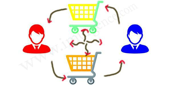
Figure 1: Factors effecting the choice of collaborative filtering
The type of filtering to be used in a recommender system is dependent on the system states. As you can see, in cases like Netflix, Amazon, Flipkart and YouTube we have user data as well as product content. A book title for example might be fiction or biography. If an anonymous visitor is checking a fiction title, then he might be recommended another title from the same or different genre. This is content based filtering based on the similarity parameters or dissimilarity.
On the other hand if the users' identity is mapped to product basket then we would be using collaborative filtering. This would be based on his pattern of purchases. In collaborative filtering the user and product association or the product and product association can be used. A hybrid filtering mechanism could be combination of two or many entities.
The choice of entities can have their own flavor like demographics, location and device data to state a few. Now after giving this brief background, I would come to the reason for doing Association Rule Mining.
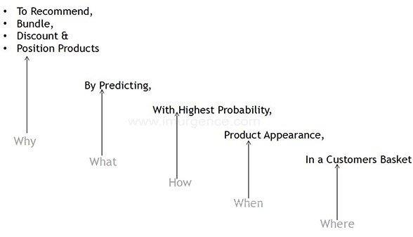
Figure 2: Association Rule Mining Objectives
We use collaborative filtering in various variants to ultimately recommend a product. As we have noted, the recommendation's are with the objective of making easy choice for customer. There is an additional commercial aspect from business perspective. It adds to the bottom line of the business. Before we look at a typical retail application of Association Rule Mining for Collaborative filtering, let do some academic implementation.
Association Rule Mining on Retail Data using R Programming
Lets do a small implementation using r codes.
We will be working on a small retail transaction dataset. Download this data file for this experiment by clicking here. Check for this data file in your local downloads folder. The file name is shopping. It would be a comma seperated file. Alternatively if you prefer working on some other dataset then you can just google it.
    # R code for association rule mining on academic data set "shopping" begins here
    # import the dataset into your rstudio or r using this code
    shopping <- read.csv("C:/Users/mohan/Downloads/shopping.csv")
The next thing after importing the data should be to observe the form of the data
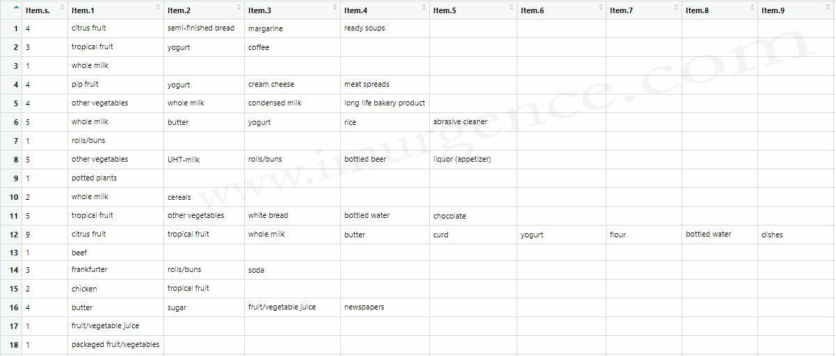
Figure 4: Snapshot of Shopping dataset imported into RStudio.
As we can see, the data has category names from a retail store. Each row has unique entries of the categories. The first column has the count of the categories from each transaction. We also observe that the customers identification and the unique transaction numbers are missing in this data. As this is an academic data set, the objective is to use the data for finding association between product categories and later use it for recommendations. We will discuss in detail how that is done at a later stage. For now, notice that the first column has count which is not something we need. We only want the category name to run the algorithm. Hence we would remove the first column having the count data.
    # Removing the unrequired 1st column named Item.s.
    shopping$Item.s. <- NULL

    # We will be using the arules package for association rule mining
    # Installing it for first time, this code will be executed only once
    # Next time you run this whole code then exclude this part as its already installed
    install.packages("arules",dependencies = TRUE)
Data Transformation
The shopping data has 9835 rows and 32 columns. We need to create a sparse matrix wherein the item name's are represented as column and transactions as rows. So each category element will be a column and its presence or absence in transaction (row) will be represented by a '0' or '1'.
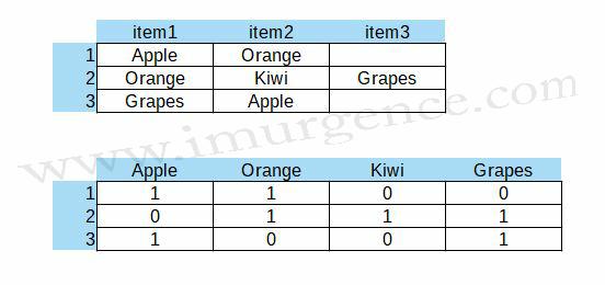
Figure 5 : Data from the first table in itemset form has to be converted into a sparse matrix format as in table below
    # load the installed arules package by calling the library function
    # library(arules)

    # count the number of rows
    nr <- nrow(shopping)

    # count the number of columns
    nc <- ncol(shopping)

    # initialize count to 1
    count=1

    # matrix initialisation
    transformed_shopping<-data.frame(matrix(nrow=0, ncol=0))

    # loop to transform the transaction data into a structure required for arules
    for (i in 1:nr)
    {
      for (j in 1:nc)
      {
        if(shopping[i,j]!="" )
        {
          transformed_shopping[count,1]<-i
          transformed_shopping[count,2]<-shopping[i,j]
          count=count+1
        }
      }
    }

    # remove the NA's if any
    transformed_shopping<-na.omit(transformed_shopping)

    # use relevent header names in the object
    colnames(transformed_shopping)<-c("trans_id","item")

    # remove duplicate entries
    transformed_shopping<-transformed_shopping[!duplicated(transformed_shopping),]

    # view the data in this form
    View(transformed_shopping)

    # convert into a sparse matrix transaction format to be ingested into the arules algorithm
    shopping_sparse <- as(split(transformed_shopping[, "item"],transformed_shopping[,"trans_id"]),"transactions")
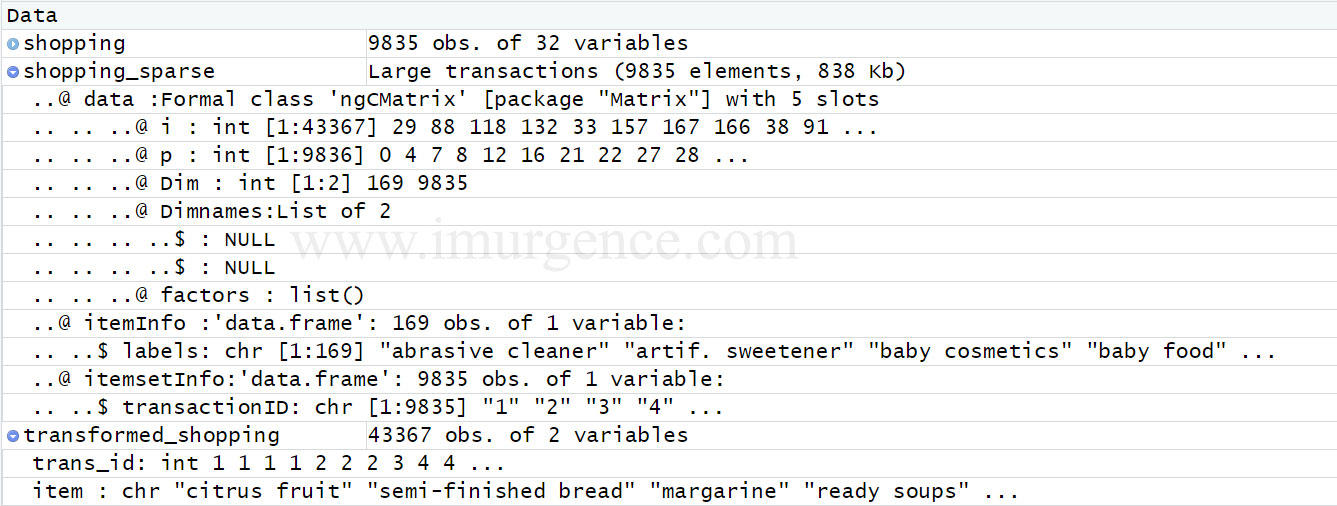
Figure 6 : Transformed data in Sparse Matrix Format
    # Lets access and check how this data looks
    shopping_sparse@data
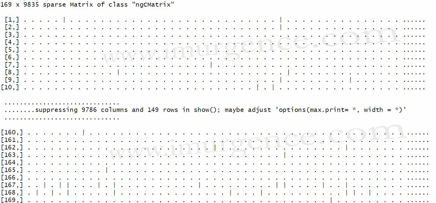
Figure 7 : Data element in the sparse matrix
As we can see the data is arranged in sparse format. Lets explore a little more, as to how the data is arranged in this format.
    shopping_sparse@itemInfo

    # run the arules algorithm, support of 0.001 means the antecedent and consequent appear together in at least 1% of transactions
    # confidence of 0.9 indicates that given the transaction had the consequent , both the antecedant & consequent were seen in those
    # transaction for more than 90 % of the time
    rules <- apriori(shopping_sparse,parameter=list(support=0.001,confidence=0.85))
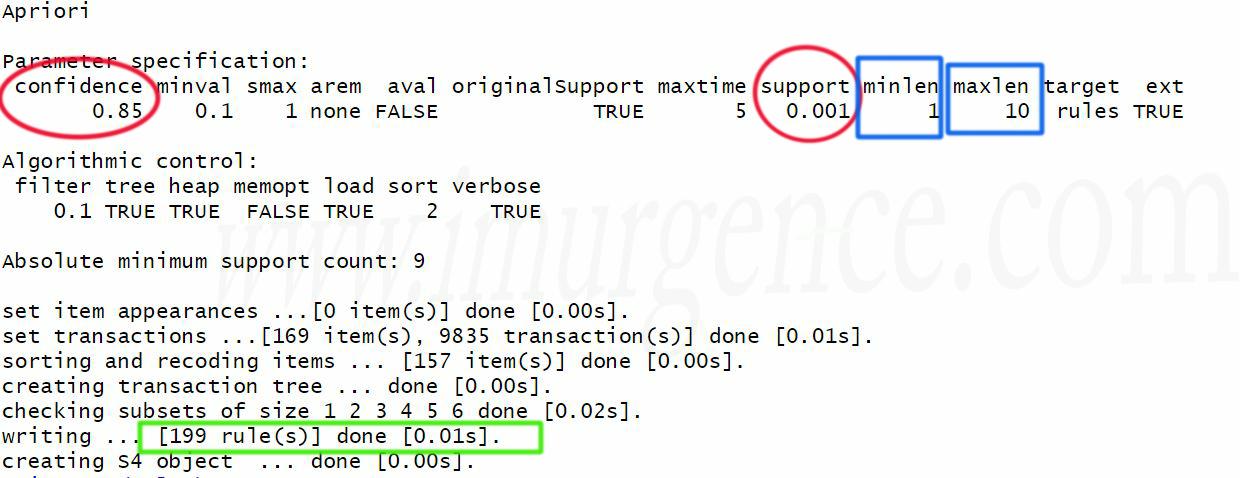
Figure 8 : Verbose Output of Apriori Algorithm
Parameters of Apriori Algorithm
As you can see, we have in red eliptical circles the support and confidence defined. Based on this parameter, for the given dataset we have excavated or mined 199 rules, marked in green box. The minlen and maxlen parameter, which is default 1 and 10 respectively. Highlighted in blue box, these can be passed as additional parameters in the call to apriori algorithm. It defines the minimum and maximum length of rule elements to be mined. Lets inspect the rules before we go ahead and sort and filter them.
  # checking the first 10 association rules of the 199 found
  inspect(rules[1:10])
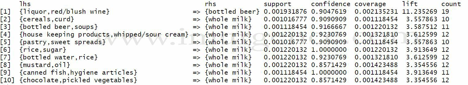
Figure 9 : First 10 Rules from the Association Rules Mined
Visualizing your Rules
    # write rules to hard disc to check manually in spreadsheet
    write(rules, file = "rules.csv", sep = ",", col.names = NA)

    # visualize your rules
    # install the "arulesViz" Package
    install.packages("arulesViz",dependencies = TRUE)

    # load the arulesViz Package to use it
    library(arulesViz)
    plot(rules,method="Grouped")
So now you have visualized your excavated rules in RStudio, as well as, you can look at the line by line elements in spreadsheet using the file on disc. If you want to have a interactive visualization of the association rules which you have created from the transactions, you will need to change some parameters in the function as below
    # plot the rules with the support representing size and lift representing shading in plot
    plot(rules,measure = "support",shading = "lift",method="grouped")

    # plot the rules with the support representing size and confidence representing shading in plot
    plot(rules,measure = "support",shading = "confidence",method="grouped")

Fig 10: Association Rule Mining Visualization using method as grouped
We can use interactive charts to explore more on the visualization as below
    # Visualization in interactive mode using engine as "interactive"
    plot(rules,measure = "support",shading = "confidence",method="grouped",engine = "interactive")
Video Demo of Interactive Visualization
Fig 11: Video of Interactive mode Visualization
Application of Collaborative Filtering in Retail Applications
While we won't go into the very details of application of Collaborative Filtering in Retail Application, we shall certainly summarize the same in flow perspective. The key note rule mining would remain pretty same with variations basis requirement. What would really be different is the data extraction and post modelling the application of rules on customer transaction basket. So the structure of expectations would typically look like this.
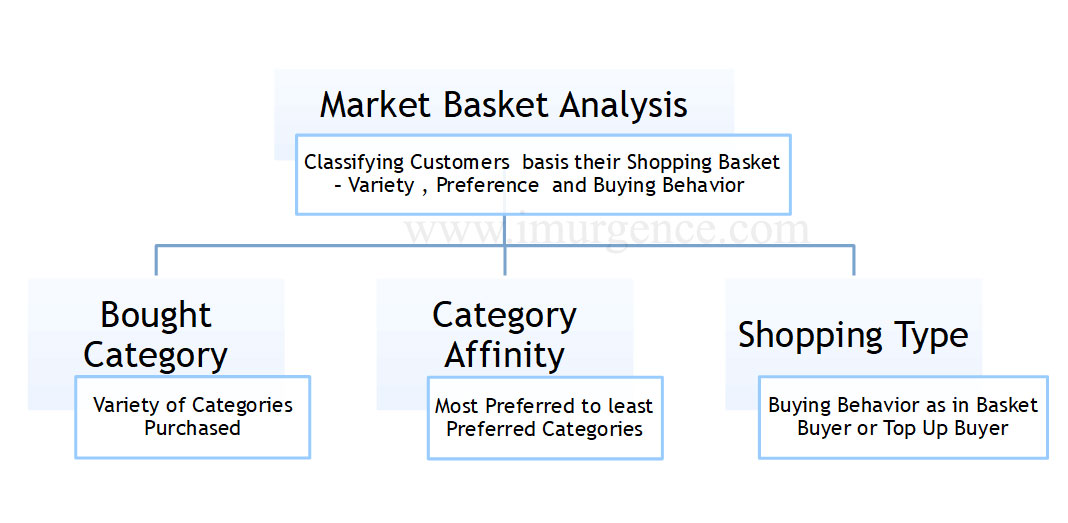
Fig 12 : Business Objectives of Collaborative Filtering
Expected Outcomes from Collaborative Filtering : Product recommendation
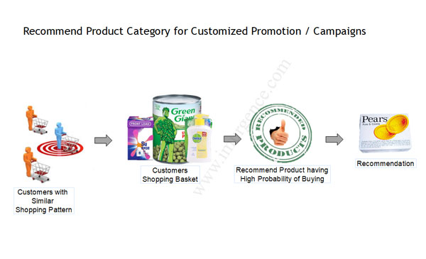
Fig 13 : Product Recommendation infographic
Expected Outcomes from Collaborative Filtering : Product Bundling
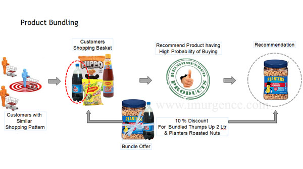
Fig 14 : Product Bundling infographic
Expected Outcomes from Collaborative Filtering : Discounting Decisions
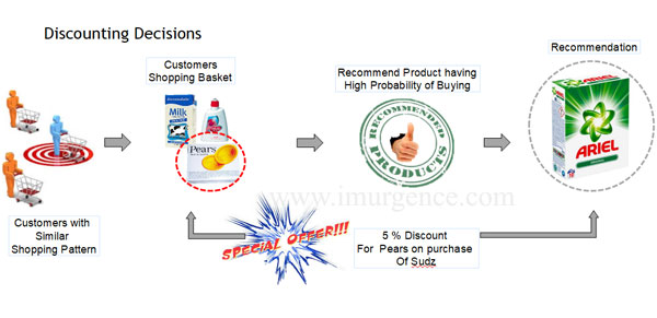
Fig 15 : Discounting infographic
Expected Outcomes from Collaborative Filtering : Product Placement
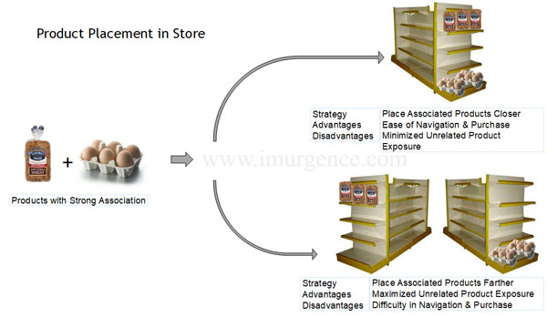
Fig 16 : Product Placement infographic
Structure of Recommendation Engine
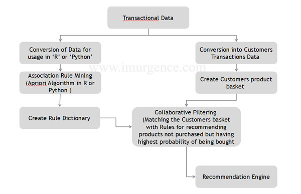
Fig 17 : Execution Work Flow
Collaborative Filtering Stage 1
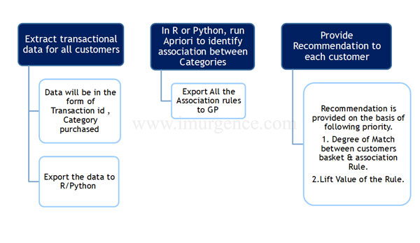
Fig 18 : Collaborative Filtering stage I
Collaborative Filtering Stage 2
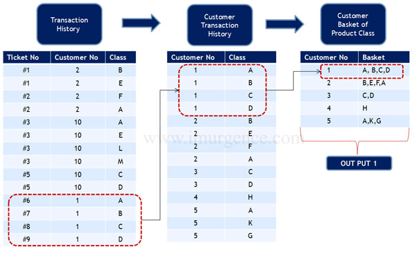
Fig 18 : Collaborative Filtering stage II
Collaborative Filtering Stage 3
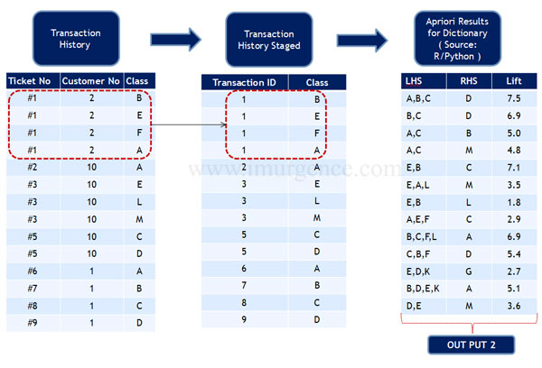
Fig 18 : Collaborative Filtering stage III
Collaborative Filtering Stage 4
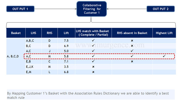
Fig 18 : Collaborative Filtering stage IV
Apriori Output Visual Explanation
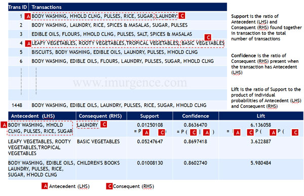
Fig 18 : Apriori Analysis Infographic
I have added an implementation of this in Python using the mlextend package as well as native python code. Do click here and check that implemenation of Association Rule Mining in Python
About the Author:
Write A Public Review