
Table of Content
- What is KNN ?
- Where do you use KNN ?
- What is K in K Nearest Neighbors ?
- How KNN works ?
- What are the distance based methods used in KNN ?
- Disadvantages of KNN
- Problem solved on Breast Cancer Dataset using KNN
- Initializing libraries
- Importing dataset
- Dataset Variable Terms Explained
- Finding missing values
- Exploratory Data Analysis
- Sorting Outlier issue
- Using Standardisation
- Splitting of Dataset to test and train
- Building KNeighbors classifier using simulation of different k values
- Building KNeighbors classifier
- Predicting for train data
- Finding the precision, recall, f1-score ,support
- Finding accuracy Score for Train Data
- Predicting Test Data
- Accuracy Score for test Data
- Pickle model as a file for usage at later stage
- Conclusion and Summary
What is KNN ?
KNN is expanded as K- Nearest Neighbors, which is a Supervised machine learning algorithm, a non -parametic method that solves both classification and regression problems. It predicts data using nearest neighbors by using distance based measures. Some distance based methods include Euclidean, Minkowsky and Manhattan.
Where do you use KNN ?
KNN is used for both Classification and Regression problems. KNN works well for small datasets and is best suitable for clinical datasets. For Classification problems, the output will be the class it belongs to and in case of Regression, the output will be the average of the values of neighbors considered.
What is the K in K Nearest Neighbors ?
The letter K is the paramter which tells the number of nearest neighbors. To predict a particular unknown point in a classification problem or regression problem, the k-value is required, which determines the number of nearest voting neighbors to find the value for the non labelled data. The K value is always a positive integer.
How KNN works ?
KNN predicts unknown value in a very interesting way ,i.e by taking the highest votes of class of its nearest neighbors. Its like telling that a person is a doctor by taking the majority votes of his nearest neighbors professions which are more of doctors than engineers. KNN algorithm finds the unkown value of data point by taking the K value of nearest neighbors and finds the distance between the points and unknown point using the given distance measure(such as Euclidean ,Minkowsky ,Manhattan or chi-sqare) .After finding the nearest neighbours by distance ,it predicts the class of unkonwn point by taking the highest number votes of the neighbor's classes. KNN doesn't learn the given dataset but simply takes it for prediction using the nearest neighbors. Hence its called the Lazy Algorithm. Just in case if the value is an unknown color, it will take majority votes as orange if the maximum number neighbors are orange and then the unkown value will be considered as orange.
The number given to k-value should always be taken into account during model building since K -value can affect accuracy and prediction and even overfitting and underfitting of data. Ideally a odd number is preferred so as to get a decision for every unlabelled data.
What are the distance based methods used in in KNN ?
Distance based methods used in KNN are Euclidean Distance, Minkowsky distance, Chisquare distance, Cosine similarity measure, Hamming distance, Chebychev distance and Mahalanobis distance. It's to be noted that the values in different variables in dataset should be scaled to unit norm before applying any distance based measure. Removal of outliers is also important, since KNN works on distance based algorithm and data points lying very faraway from the rest of the data can adversly create problem during distance measurement.
Disadvantages of KNN
- KNN cannot be used for large datasets.
- KNN doesnt learn the dataset and prediction will be always based on voting method using nearest neighbors, the prediction values wont always be correct .
- KNN will be very slow when using large amount of data.
- It is sensitive to outliers and data must be scaled to one unit.
- KNN requires huge memory for storage and processing of large datasets.
Problem solved on Breast Cancer Dataset using KNN
STEP 1 : Initializing libraries
    import pandas as pd
    import numpy as np
    import seaborn as sns
    import matplotlib.pyplot as plt
STEP 2 : Importing dataset
Click here to download the dataset.
    # use pandas read csv to ingest the downloaded data into your python environment
    data=pd.read_csv("E:\Imurgence\dataR2.csv")
STEP 3 : Dataset Variable Terms Explained
    #Age of person (years)
    #BMI of person (kg/m2)
    #Glucose level  (mg/dL)-Concentration of blood sugar in Humans Average blood sugar is 70 and 126 mg/dl.
    #Insulin level (µU/mL)-Insulin is a hormone produced by cells in Pancreas to control the amount of glucose(a type of sugar)flow in the blood and its absorption by the body .Normal Fasting Insulin level is 5 and 15 µU/mL.
    #HOMA  Homeostatic model assessment
    #Leptin (ng/mL)  It helps inhibit hunger and regulate energy balance, so the body does not trigger hunger responses when it does not need energy.
    #Adiponectin (µg/mL) Adiponectin is a protein hormone and adipokine.It is involved in regulating glucose levels and fatty acid breakdown. In humans it is encoded by the ADIPOQ gene and it is produced in primarily in adipose tissue, but also in muscle, and even in the brain.
    #Resistin (ng/mL)-Resistin increases bad cholestrol in the liver. This results in heart disease.
    #MCP-1(pg/dL) Monocyte chemoattractant protein-1 (MCP-1/CCL2) is one of the key chemokines that regulate migration and infiltration of monocytes/macrophages.

    #Classification Labels:
    #1 for Healthy controls
    #2 for Patients

    data
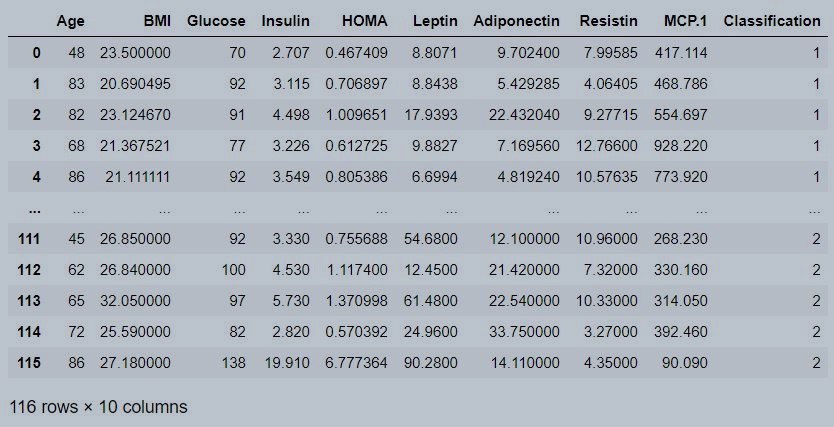
Figure 1 : Coimbra data set
    #Data Set no of rows and columns
    print(len(data),len(data.columns))
116 10
STEP 4 : Finding missing values
data.isna().sum()
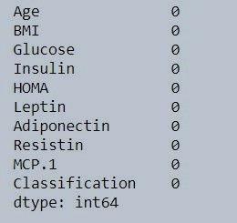
Figure 2 : Check missing value in data set
STEP 5 : Exploratory Data Analysis
    #Type of Data in Each Variable
    data.info()
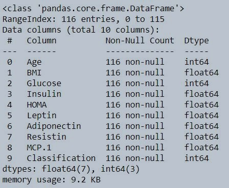
Figure 3 : Data type of individual variables in coimbra dataset
Is multicollinearity a problem in KNN?
KNN is a non-parametic method and muticollinearity is not part of the assumptions here .The heat map shown below shows the correlation among the independent variables in the dataset .We are not going to consider multicollinearity as we go ahead.
    #Heatmap to find correlation
    plt.subplots(figsize=(20,20))
    sns.heatmap(data.corr(),cmap='RdYlGn',annot=True)
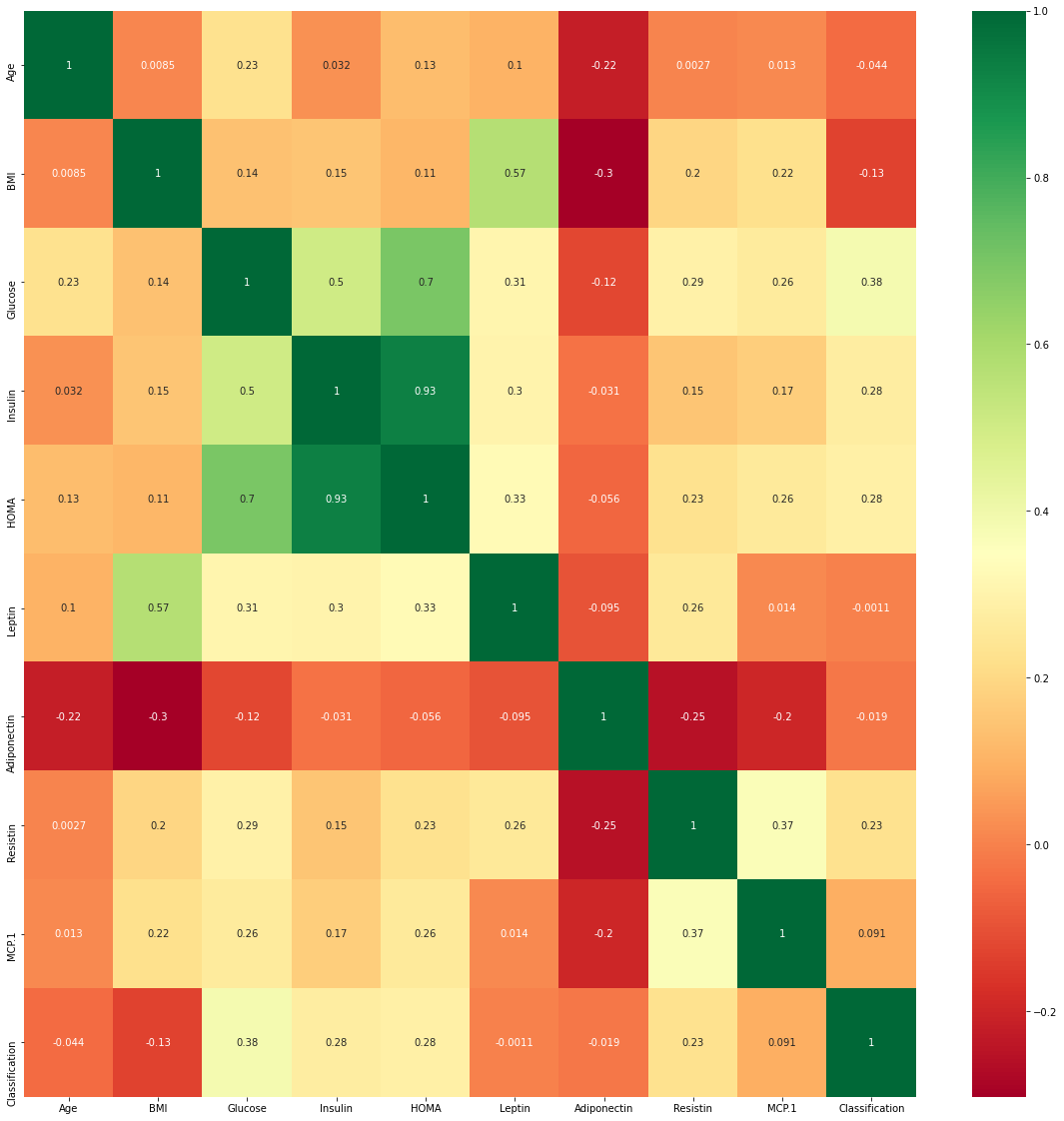 Figure 4 : Visualization of the Correlation grid
    #column Values
    data.columns
Index(['Age', 'BMI', 'Glucose', 'Insulin', 'HOMA', 'Leptin', 'Adiponectin',
       'Resistin', 'MCP.1', 'Classification'],
      dtype='object')
STEP 6 : Sorting Outlier issue
As we discussed earlier KNN is adversly affected by outliers since its a distance based measure.Now Finding outliers and to reduce them since they might affect prediction on increase in variability since we are using distance based measure.
    #No outliers for age
    sns.boxplot(data['Age'])
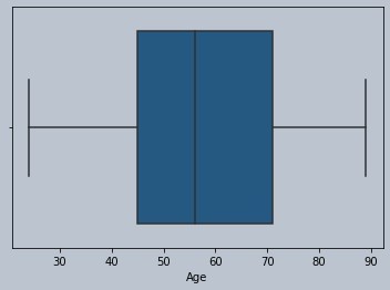 Figure 5 : Boxplot of age
    #NO outliers for BMI
    sns.boxplot(data['BMI'])
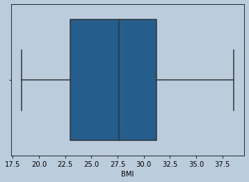 Figure 6 : Boxplot of BMI
    #Some outliers are there for Glucose and  data is Skewed
    sns.boxplot(data['Glucose'])
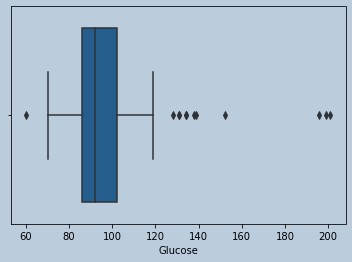 Figure 7 : Boxplot of Glucose
    #Outliers are present in Insulin
    sns.boxplot(data['Insulin'])
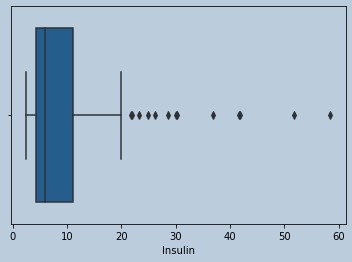 Figure 8 : Boxplot of Insulin
    #lots of Outliers in Homa
    sns.boxplot(data['HOMA'])
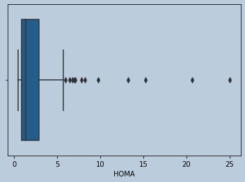 Figure 9 : Boxplot of HOMA
    #Distribution plot of HOMA
    sns.distplot(data['HOMA'])
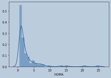 Figure 10 : Distribution plot of HOMA
    #Outliers present for Leptin
    sns.boxplot(data['Leptin'])
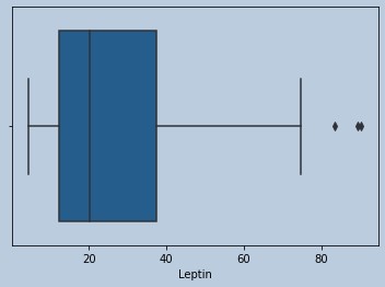 Figure 11 : Boxplot of Leptine
    #Outliers present for Adiponectin
    sns.boxplot(data['Adiponectin'])
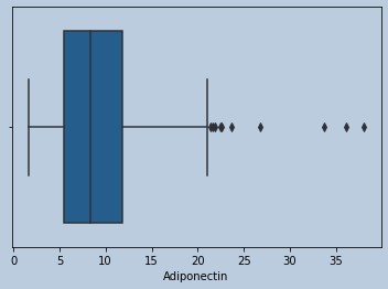 Figure 12 : Boxplot of Adiponectin
    #Ouliers present for Resistin
    sns.boxplot(data['Resistin'])
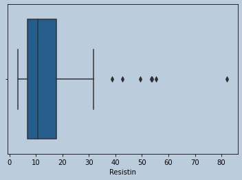 Figure 13 : Boxplot of Resistin
    #Outliers present for MCP.1
    sns.boxplot(data['MCP.1'])
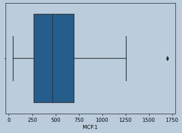 Figure 14 : Boxplot of MCP
    #Removing Outliers Since they may affect prediction for KNN (quantile method)
    cancer=data.copy()

    insulinQ1=cancer['Insulin'].quantile(0.25)
    insulinQ3=cancer['Insulin'].quantile(0.75)
    insulinIQR=insulinQ3-insulinQ1
    lowerliminsulin=insulinQ1-1.5*insulinIQR
    upperliminsulin=insulinQ3+1.5*insulinIQR
    insulrem=cancer[(cancer['Insulin']>lowerliminsulin)&(upperliminsulin > cancer['Insulin'])]


    sns.boxplot(insulrem['Glucose'])
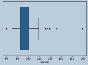 Figure 15 : Boxplot of Glucose in censored Insuline outliers
    glucoseQ1=insulrem['Glucose'].quantile(0.25)
    glucoseQ3=insulrem['Glucose'].quantile(0.75)
    glucoseIQR=glucoseQ3-glucoseQ1
    upperlimglucose=glucoseQ3+1.5*glucoseIQR
    lowerlimglucose=glucoseQ1-1.5*glucoseIQR
    glucoserem=insulrem[(insulrem['Glucose'] > lowerlimglucose)&(upperlimglucose > insulrem['Glucose'])]

    sns.boxplot(glucoserem['HOMA'])
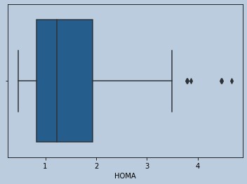 Figure 16 : Boxplot of HOMA in censored Glucose outliers
    homaQ1=glucoserem['HOMA'].quantile(0.25)
    homaQ3=glucoserem['HOMA'].quantile(0.75)
    homaIQR=homaQ3-homaQ1
    upperlimhoma=homaQ3+1.5*homaIQR
    lowerlimhoma=homaQ1-1.5*homaIQR
    homarem=glucoserem[(glucoserem['HOMA'] > lowerlimhoma)&(upperlimhoma > glucoserem['HOMA'])]

   sns.boxplot(homarem['Adiponectin'])
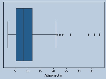 Figure 17 : Boxplot of Adiponectin in censored HOMA outliers
    AdiponectinQ1=homarem['Adiponectin'].quantile(0.25)
    AdiponectinQ3=homarem['Adiponectin'].quantile(0.75)
    AdiponectinIQR=AdiponectinQ3-AdiponectinQ1
    upperlimAdiponectin=AdiponectinQ3+1.5*AdiponectinIQR
    lowerlimAdiponectin=AdiponectinQ1-1.5*AdiponectinIQR
    adirem=homarem[(homarem['Adiponectin'] > lowerlimAdiponectin)&(upperlimAdiponectin > homarem['Adiponectin'])]

    sns.boxplot(adirem['Resistin'])
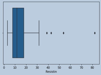 Figure 18 : Boxplot of Resistin in censored Adiponectin outliers
    resistinQ1=adirem['Resistin'].quantile(0.25)
    resistinQ3=adirem['Resistin'].quantile(0.75)
    resistinIQR=resistinQ3-resistinQ1
    lowerlimresistin=resistinQ1-1.5*resistinIQR
    upperlimresistin=resistinQ3+1.5*resistinIQR
    Resistinrem=adirem[(adirem['Resistin'] > lowerlimresistin)&(upperlimresistin > adirem['Resistin'])]

    sns.boxplot(Resistinrem['Leptin'])
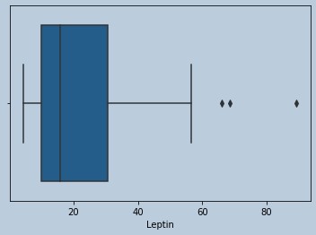 Figure 19 : Boxplot of Leptin in censored Resistin outliers
    LeptinQ1=Resistinrem['Leptin'].quantile(0.25)
    LeptinQ3=Resistinrem['Leptin'].quantile(0.75)
    LeptinIQR=LeptinQ3-LeptinQ1
    lowerlimLeptin=LeptinQ1-1.5*LeptinIQR
    upperlimLeptin=LeptinQ3+1.5*LeptinIQR
    leptinrem=Resistinrem[(Resistinrem['Leptin'] > lowerlimLeptin)&(upperlimLeptin > Resistinrem['Leptin'])]

    sns.boxplot(leptinrem['MCP.1'])
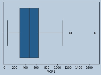 Figure 20 : Boxplot of MCP in censored Leptin outliers
    MCPQ1=leptinrem['MCP.1'].quantile(0.25)
    MCPQ3=leptinrem['MCP.1'].quantile(0.75)
    MCPIQR=MCPQ3-MCPQ1
    lowerlimMCP=MCPQ1-1.5*MCPIQR
    upperlimMCP=MCPQ3+1.5*MCPIQR
    mcprem=leptinrem[(leptinrem['MCP.1'] > lowerlimMCP)&(upperlimMCP > leptinrem['MCP.1'])]
    mcprem.shape

    sns.boxplot(mcprem['MCP.1'])
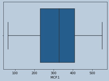 Figure 21 : Boxplot of MCP in final data
    # create the features from data
    X=mcprem.iloc[:,0:9]

    # create the target variable from data
    Y=mcprem.iloc[:,9]
STEP 7 : Using Standardisation to bring all values to one unit since KNN is a distanced based method
    from sklearn.preprocessing import StandardScaler
    ss=StandardScaler()
    X=ss.fit_transform(X)
    X=pd.DataFrame(X)
STEP 8 : Splitting of Dataset to test and train
    from sklearn.model_selection import train_test_split
    xtrain,xtest,ytrain,ytest=train_test_split(X,Y,test_size=0.3)
STEP 9 : Building KNeighbors classifier using simulation of different k values
    #Importing KNeighbors Classifier from sklearn
    #Finding accuracies  on TrainData and Test data with euclidean distance(by default p=2)
    from sklearn.neighbors import KNeighborsClassifier
    from sklearn.metrics import accuracy_score
    for x in range(5,10,2):
        knn=KNeighborsClassifier(n_neighbors=x,metric='minkowski',weights='distance')
        knn.fit(xtrain,ytrain)
        train_ypred=knn.predict(xtrain)
        acc_train_score=accuracy_score(train_ypred,ytrain)
        test_ypred=knn.predict(xtest)
        acc_test_score=accuracy_score(test_ypred,ytest)
        print(f'Accuracy score for  train data and test data is {acc_train_score} and {acc_test_score} respectively for {x} neighbours')
Accuracy score for train data and test data is 1.0 and 0.7142857142857143 respectively for 5 neighbours
Accuracy score for train data and test data is 1.0 and 0.7857142857142857 respectively for 7 neighbours
Accuracy score for train data and test data is 1.0 and 0.7142857142857143 respectively for 9 neighbours
The Train Accuracies inferred from the above model building with odd number of neighbors (5,7,9) are all the same 100% and Test accuracies are each different for the test Data with their own highs and lows. For 5 neighbors, accuracy is 71.42% whereas for 7 neighbors, the accuracy is 78.57%. We have made a better choice of taking 7 neighbors for the model building. This example clearly shows that neighbors play a vital impact on voting and prediction.Hence choosing the right number of neighbors is important and neighbors should always be an odd number.
STEP 10 : Building KNeighbors classifier using Eucledian Distance and 7 neighbors as optimal
    knn=KNeighborsClassifier(n_neighbors=7,metric='minkowski',weights='distance')
    knn.fit(xtrain,ytrain)
STEP 11 : Predicting for train data
trainypred=knn.predict(xtrain)
STEP 12 : Finding the precision, recall, f1-score ,support
    from sklearn.metrics import classification_report
    print(classification_report(trainypred,ytrain))
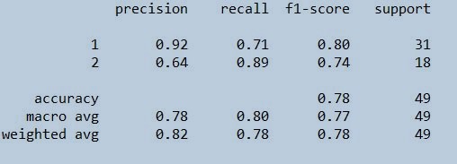
Figure 22 : Classification report on train data set
STEP 13 : Finding accuracy Score for Train Data
    accuracy_score(trainypred,ytrain)

1.0
STEP 14 : Predicting Test Data
testypredicted=knn.predict(xtest)
STEP 15 : Accuracy Score for test Data
    from sklearn.metrics import accuracy_score
    accuracy_score(testypredicted,ytest)
0.7857142857142857
STEP 16 : Pickle model as a file for usage at later stage
    import pickle
    #Save our model as a pickle to a file
    pickle.dump(knn, open("my_knn_model.pickle.dat", "wb"))

    # delete the existing knn model from the environment
    del knn

    #Load the pickled object from the file
    load_knn=pickle.load(open("my_knn_model.pickle.dat", "rb"))

    # Use the loaded model to make predictions
    load_knn.predict(xtest)
Conclusion and Summary
As you can see that the data set taken is a small clinical dataset which has got less than 150 values and is very much suitable for building KNN model. There were so many outliers in almost all the independent variables which had to be removed. We scaled the dataset before model building. Then the model was built using 6 nearest neighbours with distance measure taken as Euclidean. We got the accuracy of train and test data as 100% and 78.57% respectively. Also note that we haven't specified the seed while we were doing the split in the data set. So the train and test sets would have different instances or records. Acordingly your accurracy and precision would vary. The precision and recall for the classes stands on good score. To learn more about the subject in detail, recommend to go through these free video courses. Here we should always consider to take the best value of K for best accuracy and avoiding overfitting or underfitting of dataset.You can insert different k values and use different distance methods to get to the best optimised model. Remember to use KNN for small datasets and its good to use other parametric or non-parametric models for large datasets.
About the Author's:
Write A Public Review