
In this blog, you will get to know about various kinds of methods to deal with categorical data in a dataset, technically called as Encoding Techniques. Machine learning algorithms involve mathematical techniques to perform operations on the data and hence most of the algorithms operate on numerical data only. Since many machine learning algorithms accept only numerical values, therefore it becomes very important to convert categorical data (primarily in string form) into numerical data.
Table of Content
- Types of categorical data
- One Hot Encoding
- Dummy Encoding
- One Hot Encoding with Multiple Categories
- Label Encoding
- Ordinal Encoding
- Frequency Encoding
- Target or Mean Encoding
- Conclusion
Categorical Data
Categorical data is usually represented as strings or texts. For Example:
- Gender of a person :::: Male, Female, Others
- Educational Qualifications :::: High School, Bachelors, Masters, PhD
- States in a country :::: Delhi, UP, Haryana, Punjab etc.
- Colors :::: Red, Yellow, Orange
Primarily, we have two types of categorical data:
Nominal Data: This type of data includes multiple categories irrespective of their order. For Example:
- Colors :::: Red, Yellow, Orange
- Countries :::: India, Pakistan, China
Here, we are not concerned with the order of the categories.
Ordinal Data: This type of data includes multiple categories where ordering is important. For Example :
- Educational Qualifications :::: High School, Diploma, Bachelors, Masters, PhD
- Level of temperature :::: High, Medium, Low
Here, we can observe, the categories can be arranged in order of their priority. For example, we can give more importance to a person who has PhD degree than masters and similarly Maters will be having more weight than Bachelors.
One Hot Encoding
One hot encoding is applied when the features are nominal, that is, the order is not important. Each category is split into different columns and mapped with binary values 1 and 0. Here, 1 represents presence and 0 represents absence of that feature.
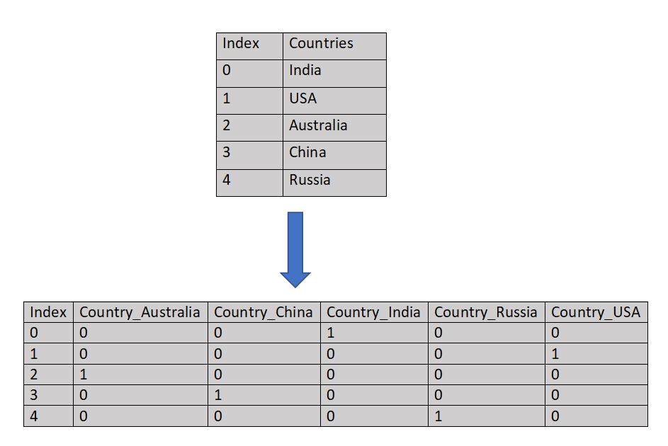
Figure 1 : One Hot Encoding Pictorial Reference
After encoding, we can see in the above table, each category of feature “Country” is represented as a separate feature where 1 value is assigned when the category is present and 0 when the category is absent.
Let’s see how to code this in Python
    # Importing the necessary library
    import pandas as pd
    import numpy as np

    # Creating a data frame using pandas
    df = pd.DataFrame({'Countries':['India','USA','Australia','China','Russia']})
    df

   Countries
0      India
1        USA
2  Australia
3      China
4     Russia

    # Importing OneHotEncoder from sklearn
    from sklearn.preprocessing import OneHotEncoder


    # Creating an instance of OneHotEncoder
    one_hot_encoder = OneHotEncoder()

    # fitting and transforimng the column to an array
    df_new = one_hot_encoder.fit_transform(df[['Countries']]).toarray()

    #Converting the array to a dataframe
    df_new = pd.DataFrame(df_new,columns=['Countries_Australia', 'Countries_China', 'Countries_India',
            'Countries_Russia', 'Countries_USA'])

    df_new.head()

   Countries_Australia  Countries_China  ...  Countries_Russia  Countries_USA
0                  0.0              0.0  ...               0.0            0.0
1                  0.0              0.0  ...               0.0            1.0
2                  1.0              0.0  ...               0.0            0.0
3                  0.0              1.0  ...               0.0            0.0
4                  0.0              0.0  ...               1.0            0.0

[5 rows x 5 columns]
Dummy Encoding
Dummy encoding is similar to one hot encoding but it creates n-1 columns after encoding, where n is the number of categories, while in one hot encoding we have n columns.
    df = pd.get_dummies(df,drop_first=True)
    df

   Countries_China  Countries_India  Countries_Russia  Countries_USA
0                0                1                 0              0
1                0                0                 0              1
2                0                0                 0              0
3                1                0                 0              0
4                0                0                 1              0
Dummy Variable Trap
Suppose you have three categories in a column namely “Male”, “Female” and “Other”. After performing One Hot Encoding, there will be three additional columns in the dataset. But only two columns are enough to predict the class of third column. For example, in this case, a person, who is neither male nor female, will definitely be in “Other” category. So, we can drop one column. It helps in better performance of model as the data gets reduced. One of the major disadvantages associated with One Hot Encoding and Dummy Encoding is: These encoding techniques create a lot of features (curse of dimensionality) in the data set which makes the model slow and computationally inefficient. For example, if we have pin codes in the data set, then it will be quite difficult to deal with huge number of encoded categories of pin codes. So, there is another technique to deal with multiple categories in a dataset which we will discuss further.
One Hot Encoding With Multiple Categories
We can use one hot encoding or dummy encoding when multiple categorical data is present in a column. For Example, if we have many Pin codes or country categories in a column then simply applying One Hot Encoding or Dummy Encoding will create huge number of encoded features. This will increase the complexity of model and make it computationally inefficient. One way to deal with such problem is using the more frequent categories in the column and encoding them into binary form (0 or 1). We can take 10-12 categories which have occurred most frequently and fit the model using those features. Here’s how this will be done: I am using Mercedes Benz dataset from Kaggle which contains various features and multiple categorical data. I have used only 6 columns from the dataset to show how this technique is applied.
    # Reading the dataset
    df = pd.read_csv(r"C:\Users\sauhard\Downloads\mercedes-benz-greener-manufacturing\train.csv",
                   usecols=['X1','X2','X3','X4','X5','X6'])
    df

     X1  X2 X3 X4  X5 X6
0     v  at  a  d   u  j
1     t  av  e  d   y  l
2     w   n  c  d   x  j
3     t   n  f  d   x  l
4     v   n  f  d   h  d
 ..  .. .. ..  .. .. ..
4204  s  as  c  d  aa  d
4205  o   t  d  d  aa  h
4206  v   r  a  d  aa  g
4207  r   e  f  d  aa  l
4208  r  ae  c  d  aa  g

[4209 rows x 6 columns]


    # Printing the number of categories in each column
    for col in df.columns:
        print(col,":",len(df[col].unique()),'labels')

X1 : 27 labels
X2 : 44 labels
X3 : 7 labels
X4 : 4 labels
X5 : 29 labels
X6 : 12 labels

    # Dummy Encoding
    pd.get_dummies(df,drop_first=True).shape

(4209, 117)

    # Frequency of each category in column X2
    df['X2'].value_counts()

as    1659
ae     496
ai     415
m      367
ak     265
.        .
.        .
.        .
o        1
af       1
ar       1
am       1
Name: X2, dtype: int64
    # Extracting top 10 most frequent features
    top_10 = [x for x in df['X2'].value_counts().head(10).index]
    top_10

['as', 'ae', 'ai', 'm', 'ak', 'r', 'n', 's', 'f', 'e']

    # Performing Encoding using Numpy
    for label in top_10:
        df[label]=np.where(df['X2']==label,1,0)

    df[['X2']+top_10]

      X2  as  ae  ai  m  ak  r  n  s  f  e
0     at   0   0   0  0   0  0  0  0  0  0
1     av   0   0   0  0   0  0  0  0  0  0
2      n   0   0   0  0   0  0  1  0  0  0
3      n   0   0   0  0   0  0  1  0  0  0
4      n   0   0   0  0   0  0  1  0  0  0
  ..  ..  ..  .. ..  .. .. .. .. .. ..  ..
4204  as   1   0   0  0   0  0  0  0  0  0
4205   t   0   0   0  0   0  0  0  0  0  0
4206   r   0   0   0  0   0  1  0  0  0  0
4207   e   0   0   0  0   0  0  0  0  0  1
4208  ae   0   1   0  0   0  0  0  0  0  0

[4209 rows x 11 columns]
We can perform this encoding technique on the remaining columns in same way. This technique extracts the most important categories, converts them into binary numbers and, hence reduces the dimension of the dataset. Therefore, our machine learning model can perform faster and better.
Label Encoding
In label encoding, each category is assigned a value from 0 to n, where n is number of category present in the column.
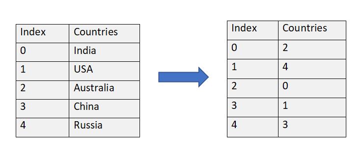
Figure 2 : Label Encoding Pictorial Reference
Let’s see how to do it in Python.
    # Creating the dataframe
    df = pd.DataFrame({'Countries':['India','USA','Australia','China','Russia']})
    df

   Countries
0      India
1        USA
2  Australia
3      China
4     Russia


    from sklearn.preprocessing import LabelEncoder
    lb = LabelEncoder()
    df['Countries'] = lb.fit_transform(df['Countries'])
    df

   Countries
0          2
1          4
2          0
3          1
4          3
Here, we can see, a random assignment of values has been done to each category. There is no specific order so that values are assigned in alphabetical ordered way. This is the major disadvantage with label encoding.
Ordinal Encoding
The ordinal encoding includes converting categorical features to numerical features considering the order or their weights i.e., more importance(numerically) will be given to more important categories.
For example, we have a feature which considers educational qualifications of a person and we want to predict salary based upon this. So, we will give more importance to a person who has a higher degree i.e.
Order of degrees :::: PhDs > Masters > Bachelors > Diploma > High school
Order of Assigned value :::: 5 > 4 > 3 > 2 > 1
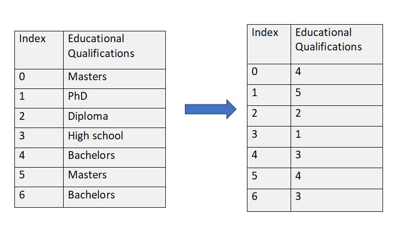
Figure 2 : Ordinal Encoding Pictorial Reference
The steps involved for performing ordinal encoding are:
- Creating a dictionary to assign values in order of importance of categories.
- Mapping each value to corresponding category in the column using map function.
    # Creating the dataframe
    df = pd.DataFrame({'Educational Qualifications':['Masters','PhD','Diploma','High school','Bachelors','Masters','Bachelors']})
    df

  Educational Qualifications
0                    Masters
1                        PhD
2                    Diploma
3                High school
4                  Bachelors
5                    Masters
6                  Bachelors

    # Assigning values to each category in order of their importance using dictionary
    dict1 = {'High school':1,'Diploma':2,'Bachelors':3,'Masters':4,'PhD':5}
    dict1

{'High school': 1, 'Diploma': 2, 'Bachelors': 3, 'Masters': 4, 'PhD': 5}

    # Mapping the dictionary to the Educational Qualification column
    df['Educational Qualifications'] = df['Educational Qualifications'].map(dict1)
    df

   Educational Qualifications
0                           4
1                           5
2                           2
3                           1
4                           3
5                           4
6                           3
Ordinal Encoding involves manual assignment of values according to categorical importance i.e., converting categorical data into numerical data through dictionary assignment.
Frequency or Count Encoding
In frequency encoding, a category is replaced by its count in the column. It’s easy to use and doesn’t increase feature space but it provides same weight if the frequencies are same.
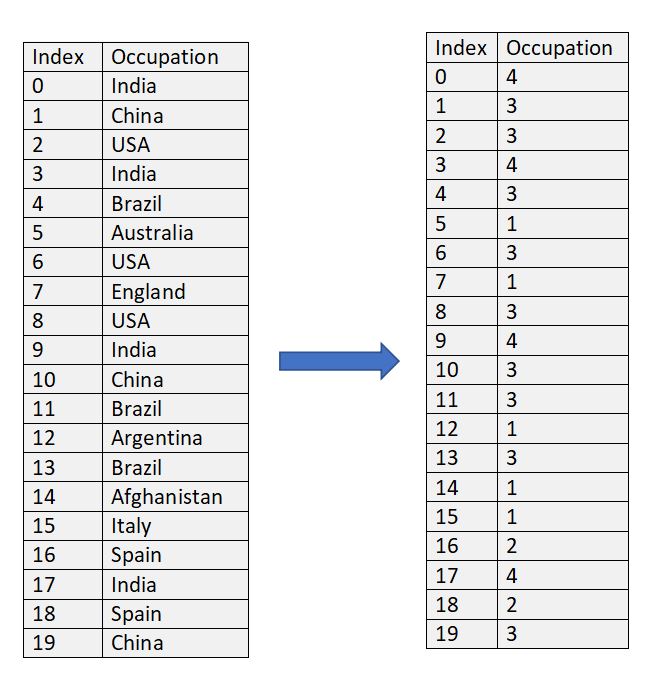
Figure 3 : Frequency or Count Encoding Pictorial Reference
Let’s see how this will be done in python.
    # Creating a dataframe
    df = pd.DataFrame({'Countries':['India','China','USA','India','Brazil','Australia','USA','England','USA','India','China',
                               'Brazil','Argentina','Brazil','Afghanistan','Italy','Spain','India','Spain','China']})
    df

      Countries
0         India
1         China
2           USA
3         India
.            ..
.            ..
16        Spain
17        India
18        Spain
19        China


    df['Countries'].value_counts()

India          4
Brazil         3
USA            3
China          3
Spain          2
Australia      1
Argentina      1
Italy          1
Afghanistan    1
England        1
Name: Countries, dtype: int64

    # Converting the value count into dictionary.
    country_count = df['Countries'].value_counts().to_dict()

    # mapping it with the feature "Countries".
    df['Countries'] = df['Countries'].map(country_count)

    df['Countries']

0     4
1     3
2     3
3     4
.     .
.     .
16    2
17    4
18    2
19    3
Name: Countries, dtype: int64
Target or Mean Encoding
Target or Mean encoding is similar to label encoding, except here labels are directly correlated with the target. We use mean of target variable to replace each category. It doesn’t affect the volume of data and hence makes learning faster. Here’s how it will be done in python.
    # Creating a dataframe
    df = pd.DataFrame({'Countries':['India','China','USA','India','Brazil','Australia','USA','England','USA','India','China',
                               'Brazil','Argentina','Brazil','Afghanistan','Italy','Spain','India','Spain','China'],
                 'Target':[1,1,0,1,0,1,0,1,0,1,0,1,1,0,0,1,1,0,1,0]})
    df

      Countries  Target
0         India       1
1         China       1
2           USA       0
3         India       1
4        Brazil       0
.           ...       .
.           ...       .
16        Spain       1
17        India       0
18        Spain       1
19        China       0


    # Calculating mean of target variable considering countries.
    df.groupby('Countries')['Target'].mean()

Countries
Afghanistan    0.000000
Argentina      1.000000
Australia      1.000000
Brazil         0.333333
China          0.333333
England        1.000000
India          0.750000
Italy          1.000000
Spain          1.000000
USA            0.000000
Name: Target, dtype: float64
Conclusion
In a nutshell, encoding categorical data is necessary part of data pre-processing, though there isn’t any specific method which you can apply for a particular problem. It all depends on your requirements i.e., the problem and dataset. You can try different methods for the problem and find out which work best according to the requirements. Recommend to read this interesting article on Logistic Regression for MNIST digit classification in Python.
About the Author's:
Write A Public Review