
Table of Content
- About Survival Analysis.
- Terms Used in Survival Analysis.
- Types of Survival Analysis.
- Kaplan-Meier Estimator.
- Cox Proportional Hazards Regression analysis.
- About Dataset.
- Implementation of Survival Model
- Conclusion
About Survival Analysis
Before creating survival analysis model we have to understand what is survival analysis and how it can help us. So, survival analysis is a branch of statistics which helps in modeling the time that a particular event may take to occur. With the help of survival analysis we can give the answers of many questions, like when the machine system failure will take place, survival time of patients affected by disease and how much time it will take to cure the disease. It is also helpful in insurance sector as it can predict the survival of policy holder or actuaries fix an appropriate insurance premium in underwriting.
Terms Used in Survival Analysis
Events : It is the activity which is currently going on or going to happen like death of a person from disease, time taken to cure from disease, time taken to cure by vaccine, failure of machines, etc.
Time : It is a time taken from beginning of the observation to the end of it or we can say till the time when event is going to happen.
Censoring or Censored Observation : If the subject on which we are doing survival analysis doesn’t get affected by the defined event is known as censored. A censored subject may or may not have any event after the end of observation time.
There are three types of Censoring:
Right Censored : If we are not sure what happened to subject after certain point in time it is known as Right Censored. Its main reason is that the actual event time is greater than the censored time.
Ex: A patient who has not been cured at the time of observation
Left Censored : If we are not sure what happened to subject before certain point of time is known as Left Censored. Its main reason is that the actual event time is less than the censored time.
Interval Censored : If we are sure that event has occurred in a time interval but don’t know when it is actually occurred is known as Interval Censored.
Survival Function : It is the probability function that depends upon the time “t” of the study. The survival function gives the probability that the subject survived more than time “t”.
Types of Survival Analysis
The process of survival analysis can be performed through various techniques like:
- Kaplan-Meier Estimator
- Cox Proportional Hazards Regression Analysis
- Survivors and Hazards function rate
- Survival Tree
- Survival Random Forest
- Parametric survival analytic model
In this article we will talk about Kaplan-Meier estimator and Cox Proportional Hazards regression analysis.
Kaplan-Meier Estimator
It is a non-parametric statistic used to estimate person surviving probability (survival function) from lifetime data. For example, survival time of patient after the diagnosis or from the time when the treatment starts.
It is one of the most used methods of survival analysis. The estimate may be useful to examine the probability of death or the recovery rate.
Three assumptions must be made before using Kaplan-Meier estimator:
- Subjects that are censored have the same survival prospects as those who continue to be followed.
- Survival probability is the same for all the subjects.
- The event of interest happens at the specified time. The estimated survival time can be more accurately measured if the examination happens frequently.
The visual representation of this function is known as Kaplan-Meier Curve.
Mathematically Kaplan-Meier estimator represented as below:
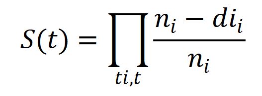
ni = number of subjects at risk before time t .
di = number of the desired event at time t .
Parametric survival models and the Cox proportional hazards model may be useful to estimate covariate-adjusted survival rather than Kaplan-Meier estimator.
Cox Proportional Hazards Regression analysis
It is basically a regression model commonly used in healthcare to investigate the relation between survival time of patients with other variables.
Where Kaplan-Meier estimator is used for univariate analysis, Cox proportional hazards is used for multivariate analysis.
It is expressed by the hazard function denoted by h(t) and it can be interpreted as the risk of dying at time t.
Mathematically it will be represented as:
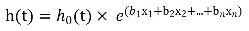
where,
t = survival time,
h(t) = hazard function determined by a set of n covariates,
h0 = baseline hazard.
The exponential expression called as Hazard Ratio(HR), if its value is greater than 1 it will indicate a covariate that is positively correlated with event probability which mean it is negatively correlated with survival length.
If,
HR > 1: Increase in Hazards
HR = 1: No effect
HR < 1: Reduction in Hazards
Let’s see how to build the survival analysis model using Haberman’s Survival dataset.
About Dataset
The dataset contains a set of 306 patients whose survival time is given in years from 1958 to 1970. It contains 4 features:
Age of patient at time of operation as Age.
Patient’s year of operation as Year_of_Operation.
No. of positive axillary nodes detected as Axillary_nodes.
Survival status :
1 = Patient survive 5 years or longer.
2 = Patient died within 5 years.
Download survival data set by clicking here
Implementation of Survival Model
First we have to install lifelines library which contains survival analysis models.
    # Importing Libraries
    import numpy as np
    import pandas as pd
    import matplotlib.pyplot as plt
    import seaborn as sns

    # Importing Dataset
    data = pd.read_excel("Survival model.xlsx")
    data.head(5)

   Patient_Age  Year_of_Operation  Axillary_nodes  Survival Status
0           30                 64               1                1
1           30                 62               3                1
2           30                 65               0                1
3           31                 59               2                1
4           31                 65               4                1

    data.info()


RangeIndex: 306 entries, 0 to 305
Data columns (total 4 columns):
 #   Column             Non-Null Count  Dtype
---  ------             --------------  -----
 0   Patient_Age        306 non-null    int64
 1   Year_of_Operation  306 non-null    int64
 2   Axillary_nodes     306 non-null    int64
 3   Survival Status    306 non-null    int64
dtypes: int64(4)
memory usage: 9.7 KB

    data.describe()

       Patient_Age  Year_of_Operation  Axillary_nodes  Survival Status
count   306.000000         306.000000      306.000000       306.000000
mean     52.457516          62.852941        4.026144         1.264706
std      10.803452           3.249405        7.189654         0.441899
min      30.000000          58.000000        0.000000         1.000000
25P      44.000000          60.000000        0.000000         1.000000
50P      52.000000          63.000000        1.000000         1.000000
75P      60.750000          65.750000        4.000000         2.000000
max      83.000000          69.000000       52.000000         2.000000
    # Lets check the distribution of the target class in the data
    data['Survival Status'].value_counts()

1    225
2     81
Name: Survival Status, dtype: int64
We will be needing the lifelines package. If you are using Jupyter Notebook then you need to
!pip install lifelines
else if you are using anaconda distribution, then open the anaconda prompt and give the following command in your terminal
    pip install lifelines --user

    # in both the cases you would be seeing the system executing a bunch of downloads and check to build your environment for survival analytics. Something like this

(base) C:\Users\Mohan Rai>pip install lifelines --user
Collecting lifelines
  Downloading lifelines-0.26.0-py3-none-any.whl (348 kB)
     |????????????????????????????????| 348 kB 3.3 MB/s
Collecting autograd>=1.3
  Downloading autograd-1.3.tar.gz (38 kB)
Requirement already satisfied: matplotlib>=3.0 in c:\users\Mohan Rai\anaconda3\lib\site-packages (from lifelines) (3.3.2)
Collecting autograd-gamma>=0.3
  Downloading autograd-gamma-0.5.0.tar.gz (4.0 kB)
Collecting formulaic<0.3,>=0.2.2
  Downloading formulaic-0.2.3-py3-none-any.whl (55 kB)
     |????????????????????????????????| 55 kB 584 kB/s
Requirement already satisfied: numpy>=1.14.0 in c:\users\Mohan Rai\anaconda3\lib\site-packages (from lifelines) (1.19.2)
Requirement already satisfied: pandas>=0.23.0 in c:\users\Mohan Rai\anaconda3\lib\site-packages (from lifelines) (1.1.3)
Requirement already satisfied: scipy>=1.2.0 in c:\users\Mohan Rai\anaconda3\lib\site-packages (from lifelines) (1.5.2)
Requirement already satisfied: future>=0.15.2 in c:\users\Mohan Rai\anaconda3\lib\site-packages (from autograd>=1.3->lifelines) (0.18.2)
Requirement already satisfied: kiwisolver>=1.0.1 in c:\users\Mohan Rai\anaconda3\lib\site-packages (from matplotlib>=3.0->lifelines) (1.3.0)
Requirement already satisfied: cycler>=0.10 in c:\users\Mohan Rai\anaconda3\lib\site-packages (from matplotlib>=3.0->lifelines) (0.10.0)
Requirement already satisfied: python-dateutil>=2.1 in c:\users\Mohan Rai\anaconda3\lib\site-packages (from matplotlib>=3.0->lifelines) (2.8.1)
Requirement already satisfied: pillow>=6.2.0 in c:\users\Mohan Rai\anaconda3\lib\site-packages (from matplotlib>=3.0->lifelines) (8.0.1)
Requirement already satisfied: pyparsing!=2.0.4,!=2.1.2,!=2.1.6,>=2.0.3 in c:\users\Mohan Rai\anaconda3\lib\site-packages (from matplotlib>=3.0->lifelines) (2.4.7)
Requirement already satisfied: certifi>=2020.06.20 in c:\users\Mohan Rai\anaconda3\lib\site-packages (from matplotlib>=3.0->lifelines) (2020.6.20)
Collecting interface-meta>=1.2
  Downloading interface_meta-1.2.3-py2.py3-none-any.whl (14 kB)
Collecting astor
  Downloading astor-0.8.1-py2.py3-none-any.whl (27 kB)
Requirement already satisfied: wrapt in c:\users\Mohan Rai\anaconda3\lib\site-packages (from formulaic<0.3,>=0.2.2->lifelines) (1.12.1)
Requirement already satisfied: pytz>=2017.2 in c:\users\Mohan Rai\anaconda3\lib\site-packages (from pandas>=0.23.0->lifelines) (2020.1)
Requirement already satisfied: six in c:\users\Mohan Rai\anaconda3\lib\site-packages (from cycler>=0.10->matplotlib>=3.0->lifelines) (1.15.0)
Building wheels for collected packages: autograd, autograd-gamma
  Building wheel for autograd (setup.py) ... done
  Created wheel for autograd: filename=autograd-1.3-py3-none-any.whl size=47994 sha256=0e2849ff4c4bf65d078d967a5a83fc7c2a9885b2d952230896f9619b2d4758f6
  Stored in directory: c:\users\Mohan Rai\appdata\local\pip\cache\wheels\85\f5\d2\3ef47d3a836b17620bf41647222825b065245862d12aa62885
  Building wheel for autograd-gamma (setup.py) ... done
  Created wheel for autograd-gamma: filename=autograd_gamma-0.5.0-py3-none-any.whl size=4039 sha256=b87332a27e0a6ed03ac0e14c99f74584a0aeff26b9f266e63a4095d7ddf6c9fb
  Stored in directory: c:\users\Mohan Rai\appdata\local\pip\cache\wheels\16\a2\b6\582cfdfbeeccd469504a01af3bb952fd9e7eccba40995eafea
Successfully built autograd autograd-gamma
Installing collected packages: autograd, autograd-gamma, interface-meta, astor, formulaic, lifelines
Successfully installed astor-0.8.1 autograd-1.3 autograd-gamma-0.5.0 formulaic-0.2.3 interface-meta-1.2.3 lifelines-0.26.0

(base) C:\Users\Mohan Rai>
    # Lets plot Kaplan-Meier Curve
    from lifelines import KaplanMeierFitter
    durations = data['Patient_Age']
    event_observed = data['Survival Status']
    kmf = KaplanMeierFitter()
    kmf.fit(durations, event_observed=event_observed)
    kmf.plot()
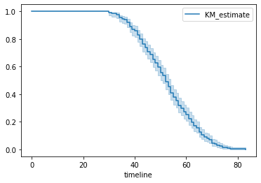
Figure 1 : Plot of Kaplan Meier Curve
In above graph, y-axis represents the probability of the subject still having not experienced the event after time t, where y = 1 means the patient is alive and y = 0 means patient didn’t survived and x-axis represents the time t.
    # creating two cohorts
    groups = data['Axillary_nodes']
    i1 = (groups >= 1)
    i2 = (groups < 1)

    kmf_2 = KaplanMeierFitter()
    ## fit the model for 1st cohort
    kmf_2.fit(durations[i1], event_observed[i1], label='at least one positive axillary detected')
    a = kmf_2.plot()

    ## fit the model for 2nd cohort
    kmf_2.fit(durations[i2], event_observed[i2], label='no positive axillary nodes detected')
    kmf_2.plot(ax=a)
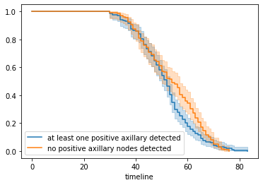
Figure 2 : Plot of Fitting Kaplan on two cohorts
From the above curve, we can say that approximately before 45 years both curve are overlapped which means a patient has high probability to survive if he is less than 45 years irrespective of surgery and for greater than 45 years, those patients who undergone through at least one surgery are more likely to not die sooner than the others who have not done any surgery yet.
    kmf_2.event_table

          removed  observed  censored  entrance  at_risk
event_at
0.0             0         0         0       136      136
30.0            1         1         0         0      136
33.0            1         1         0         0      135
34.0            2         2         0         0      134
35.0            1         1         0         0      132
..             ..        ..        ..        ..       ..
..             ..        ..        ..        ..       ..
..             ..        ..        ..        ..       ..
..             ..        ..        ..        ..       ..
70.0            4         4         0         0       11
72.0            3         3         0         0        7
73.0            2         2         0         0        4
74.0            1         1         0         0        2
76.0            1         1         0         0        1
    kmf.predict(45)

0.7091503267973858
    # Creating Cox Proportional Hazards Model
    from lifelines import CoxPHFitter
    cph = CoxPHFitter()

    # Fit the data to train the model
    cph.fit(data, 'Patient_Age', event_col='Survival Status')

    # Have a look at the significance of the features
    cph.print_summary()


             model       = lifelines.CoxPHFitter
             duration col = 'Patient_Age'
                event col = 'Survival Status'
      baseline estimation = breslow
   number of observations = 306
number of events observed = 306
   partial log-likelihood = -1446.95
         time fit was run = 2021-06-15 12:01:43 UTC

---
                    coef  exp(coef)   se(coef)   coef lower 95%   coef upper 95%  exp(coef) lower 95%  exp(coef) upper 95%
covariate
Year_of_Operation  -0.02       0.98       0.02            -0.06             0.01                 0.94                 1.01
Axillary_nodes      0.01       1.01       0.01            -0.00             0.03                 1.00                 1.03

                      z    p   -log2(p)
covariate
Year_of_Operation -1.39 0.16       2.61
Axillary_nodes     1.70 0.09       3.47
---
Concordance = 0.53
Partial AIC = 2897.90
log-likelihood ratio test = 4.50 on 2 df
-log2(p) of ll-ratio test = 3.25
    # Have a look at the significance of the features
    cph.plot()
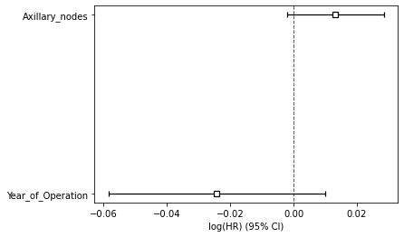
Figure 3 : Plot of Covariate Significance for Predicting Survival Risk
Above summary shows the significance of the covariates in predicting the survival risk. Both features play a significant role in predicting the survival. The large CI indicates that more data would be needed.
Now, let’s see the probability of survival at patient level.
    patient = [50,100,280]
    pred = data.iloc[patient,1:3]
As we have seen that only year of operation and axillary nodes are important for model so we have selected only these feature for prediction of survival probability. Let’s predict and visualize the probability graph.
cph.predict_survival_function(pred).plot()
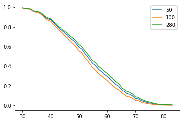
Figure 4 : Plot of Survival Prediction Function
Figure 4, shows that patient number 280 has higher chance of survival than other two patients at any time t.
Conclusion
In this article we have learnt about the theory of Survival Analysis Model and implemented it using python. We have seen survival probability using Kaplan-Meier estimator and Cox Proportional Hazards Regression Model and at last we have done prediction for random patients and seen their probability of survival at any time t. Check this interesting application of Human Pose Estimation Using OpenCV in Python.
About the Author's:
Write A Public Review