Table of Content
About Time Series Analysis
Time series analysis is a statistical method to deal with time series data or to find trends in data with respect to time.
Now a question arises what is time series data, it’s basically a data which consist series of particular time periods or intervals taken sequentially.
It consist only one variable and data is taken at various time for that variable.
If the data is taken for more than one variable at same point of time it is know as Cross-sectional data.
Terms Related to Time Series
Stationary Data : If the mean value of data remains constant over a time interval is called Stationary.
Non-Stationary Data : If mean value of data changes over a time period is called Non-stationary data.
Some examples of time series data are: temperature values, stock price, and price of house over time, etc.
Differencing : It is used to make the series stationary or to de-trend the data.
Exponential smoothing : It is used to predict the next period values based on the historical data. It involves averaging of data such that non-averaging data or component of each individual cancel out each other. It is used to predict the short term prediction.
Predicting Stock Price Using LSTM Model
LSTM stand for Long-short term memory, it is an artificial feed forward and Recurrent Neural Network (RNN) used in deep learning. It is capable of learning order dependencies in sequence prediction problems.
Its take 3 dimensions as input for prediction. It is used for classifying, image processing, video processing, speech recognition and for predictions.
We are going to predict the stock price using multi layer LSTM model
Importing necessary Libraries and Dataset
Libraries needed are Pandas, Numpy, Scikit-Learn, Plotly , Tensorflow and Keras.
    # Importing Libraries
    import pandas as pd
    import numpy as np
    import matplotlib.pyplot as plt
    import plotly.io as plt_io
    import plotly.express as px
    import plotly.figure_factory as ff
    from tensorflow import keras
    from sklearn.preprocessing import MinMaxScaler

    # read the data file (Download Data from Here)
    stock_price = pd.read_csv('Stock data.csv', parse_dates=['Date'])
    stock_price = stock_price.set_index('Date')
    stock_price.head(5)

                    Open          High  ...     Adj Close   Volume
Date                                    ...
2020-03-03  38480.890625  38754.238281  ...  38623.699219  10600.0
2020-03-04  38715.718750  38791.699219  ...  38409.480469  15300.0
2020-03-05  38604.250000  38887.800781  ...  38470.609375  13500.0
2020-03-06  37613.960938  37747.070313  ...  37576.621094  19000.0
2020-03-09  36950.199219  36950.199219  ...  35634.949219  18800.0
    # Retaining only the closing price
    stock_price = stock_price[['Close']]
    stock_price.head(5)

                   Close
Date
2020-03-03  38623.699219
2020-03-04  38409.480469
2020-03-05  38470.609375
2020-03-06  37576.621094
2020-03-09  35634.949219
Checking for Nan values and trend
After uploading the data next step is to check whether data have nan values or not and then we plot the close price on graph.
    stock_price[stock_price.isnull().any(axis=1)]

            Open  High  Low  Close  Adj Close  Volume
Date
2020-11-14   NaN   NaN  NaN    NaN        NaN     NaN
2021-01-01   NaN   NaN  NaN    NaN        NaN     NaN

    stock_price=stock_price.dropna()
We got 2 null values on 14-11-2020 and 01-01-2021 but we know that on this days due to National holidays market was closed, so actually it’s not a missing value and we can drop them.
Let’s visualize the price trend of stock. We are using the plotly module, so we are going to change the default svg to browser. Unless you do this your plots wont be visible. You will have to run these patch of code
    plt_io.renderers.default='browser'
    stock_chart=px.line(x = stock_price.index, y = stock_price['Close'], title = "Closing Price Of Stock")
    stock_chart.show()

Figure 1 : Interactive plot of Stock Data using plotly rendered on a browser
As we can see it’s not a stationary data, it follows a trend and for this type LSTM model is good for predictions.
The next step is to split the data into train and test sets to train over model.
    train_rec = int(len(stock_price) * 0.70)
    train_df = stock_price[0:train_rec]
    print(train_df.shape)

(174, 1)

    test_df = stock_price[train_rec:]
    print(test_df.shape)

(75, 1)
As our data has very high range of prices so let’s scale down them.
    sc = MinMaxScaler(feature_range = (0, 1))
    train_scaled = sc.fit_transform(train_df)
    test_scaled = sc.transform(test_df)

    def dataset(data , n_features):
        X, Y = [], []
        for i in range(len(data)-n_features-1):
            a = data[i:(i+n_features), 0]
            X.append(a)
            Y.append(data[i + n_features, 0])
        return np.array(X), np.array(Y)

    n_features = 3 # It takes previous 3 days stock price to predict next day price
    X_train, y_train = dataset(train_scaled, n_features)
    X_test, y_test = dataset(test_scaled, n_features)
Model Building
We are going to use LSTM algorithm which takes input data as 3-D. So we have to convert data into 3-D.
    X_train = X_train.reshape(X_train.shape[0] ,X_train.shape[1],1)
    X_test = X_test.reshape(X_test.shape[0] ,X_test.shape[1],1)
    print(X_train.shape , y_train.shape , X_test.shape , y_test.shape)

(170, 3, 1) (170,) (71, 3, 1) (71,)
Now we will create model with 150 neurons. One output layer for predicting stock price. We are using mean squared error loss function and adam gradient optimizer.
    # Create the model
    inputs = keras.layers.Input(shape=(X_train.shape[1], X_train.shape[2]))
    x = keras.layers.LSTM(150, return_sequences= True)(inputs)
    x = keras.layers.Dropout(0.3)(x)
    x = keras.layers.LSTM(150, return_sequences=True)(x)
    x = keras.layers.Dropout(0.3)(x)
    x = keras.layers.LSTM(150)(x)
    outputs = keras.layers.Dense(1, activation='linear')(x)

    model = keras.Model(inputs=inputs, outputs=outputs)
    model.compile(optimizer='adam', loss="mean_squared_error", metrics=['mean_squared_error'])
    model.summary()

Model: "model"
_________________________________________________________________
Layer (type)                 Output Shape              Param #
=================================================================
input_1 (InputLayer)         [(None, 3, 1)]            0
_________________________________________________________________
lstm (LSTM)                  (None, 3, 150)            91200
_________________________________________________________________
dropout (Dropout)            (None, 3, 150)            0
_________________________________________________________________
lstm_1 (LSTM)                (None, 3, 150)            180600
_________________________________________________________________
dropout_1 (Dropout)          (None, 3, 150)            0
_________________________________________________________________
lstm_2 (LSTM)                (None, 150)               180600
_________________________________________________________________
dense (Dense)                (None, 1)                 151
=================================================================
Total params: 452,551
Trainable params: 452,551
Non-trainable params: 0

    # Train model
    history = model.fit(X_train, y_train, epochs = 25 , batch_size = 60, validation_split= 0.2 )
    pred = model.predict(X_test)
    pred = sc.inverse_transform(pred)
    test_actual = y_test.reshape(X_test.shape[0] , 1)
    test_actual = sc.inverse_transform(test_actual)

    # Append the predicted values to the list
    test_predicted = []
    for i in pred:
      test_predicted.append(i[0])
    df_predicted = pd.DataFrame()
    df_predicted['Prediction'] = test_predicted
    df_predicted['Actual'] = test_actual
    df_predicted.head(5)

     Prediction        Actual
0  43248.277344  44180.050781
1  43497.429688  43599.960938
2  43822.769531  43882.250000
3  43804.261719  44077.148438
4  43559.601562  44523.019531
Visualization
We got the predicted price and actual price in a single dataframe let’s compare them by visualizing.
    def interactive_plot(df, title):
      stock_chart = px.line(title = title)
      for i in df.columns[0:]:
        stock_chart.add_scatter(x = df.index, y = df[i], name = i)
      stock_chart.show()

    interactive_plot(df_predicted, "Stock Price Predicted")
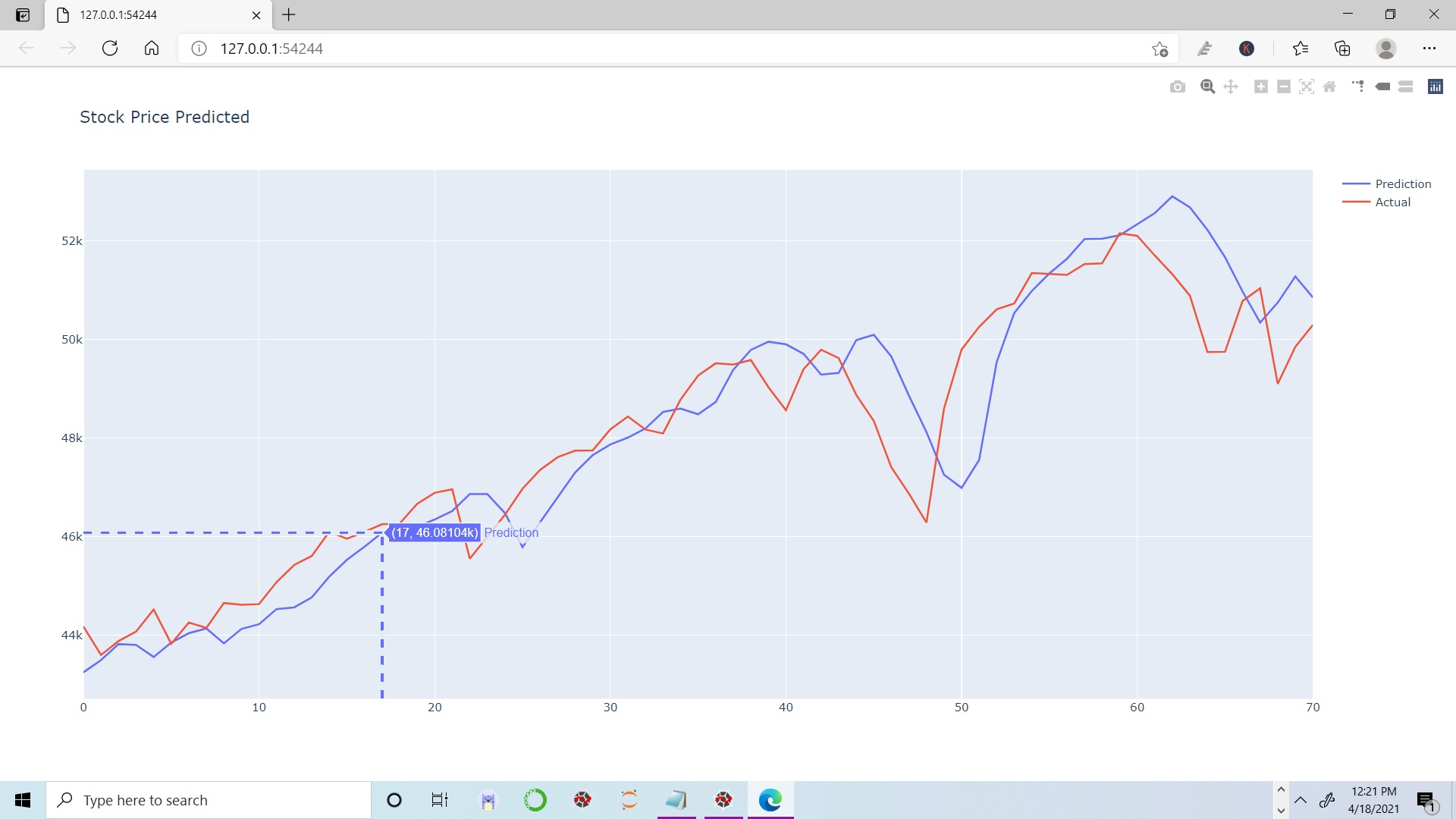
Figure 2 : Plot of Actual vs Predicted Stock Data using plotly
Summary
We can clearly see that our model worked good for recent data stamps, we can see that model predicted little higher value as compared to actual stock value. So, in this article we have learnt bout Time Series Analysis , LSTM Model and seen that how to build LSTM model for stock price prediction. And at last we have compared predicted stock price with actual price .Do read this interesting article on MNIST digit classification using Logistic Regression.
About the Author's:
Write A Public Review