
Table of Content
- Inspiration
- Dataset Description
- Dependency Packages Installing in python
- Loading Dataset
- Import Required Libraries
- Explore Dataset
- Build Model using Pycaret
- Evaluate Model
- Stack Model
- Save Model for Reuse
- Conclusion
Inspiration
The object of this project is to predict how long a car on a production line will take to pass the testing phase. Knowing that predicted time will help to reduce the time that cars spend on test bench. This would lead to increase in the production effeciency by contributing in faster testing, without disturbing standards.
This project's approach relies on building that predictive capability using machine learning and various algorithm's in order to help manufacturing industry to increase production. It's a regression problem. In this project we will explore low code pycaret library advanced techniques such as
- Dimensionality reduction PCA (Principal Componanent Analysis)
- Transforming target
- Handling of Low variance features
- Combining rare levels
- Stacking of models
Dataset Description
- Dataset contains masked features each representing a custom feature in a Mercedes car and each row represents a seperate car. For example, a variable could be 4WD, added air suspension, or a head-up display.
- Target column is 'y' which represents the time taken by car to pass test in seconds
- For validation purpose test data is available on kaggle. You can get test score by submitting the test predictions at Kaggle website where this competetion was held. But for ease of use we are going to use only the train data from Kaggle and use the test data by simulation. We have kept a copy of the train data in the Loading data section.
Dependency Packages Installing in python
We are installing packages in python by using “pip” followed by install package name. For example, write “ !pip install pycaret ” and run that tab when you are using jupyter notebook.
If you are using a editor you have to modify the script accordingly, for instance, if you are using the anaconda distribution then you can use navigator to install the package or you can use the anaconda prompt where you can type - "pip install pycaret" to install. Its better if you create a new environment in anaconda navigator or command prompt, wherein you use python 3.6 version. This would avoid disturbing your existing dependencies build for other projects.
Required packages for this project are as below:
- Pandas- to perform dataframe operations
- Numpy- to perform array operations
- Matplotlib- to plot charts
- Seaborn – to plot charts
- Missingno- anlysing the missing values
- pycaret – to build the model and save the model.
Loading Dataset
Click on this link to download the data set
Import Required Libraries
    # Lets import required libraries
    import pandas as pd
    import numpy as np
    import matplotlib.pyplot as plt
    import seaborn as sns

    import warnings
    warnings.filterwarnings('ignore')

    %matplotlib inline

    # reading the dataset
    df = pd.read_csv('mercedes-benz-production-optimization-data.csv.csv')
Explore Dataset
As our problem is related to regression we will first analyse the target dataset. We will have a look at the dataset features and see how it will help to predict the target.
df.info()
RangeIndex: 4209 entries, 0 to 4208
Columns: 378 entries, ID to X385
dtypes: float64(1), int64(369), object(8)
memory usage: 12.1+ MB
    # data the has lots of features so setting options to view all columns
    pd.options.display.max_columns = 400

    df.head() # not displaying the output in this writeup, but u may get a scrolling tab if using notebook or it may show up in editor with first 5 records

    # Visualize the target variable
    plt.scatter(range(len(df)), np.sort(df.y.values), alpha=0.3)
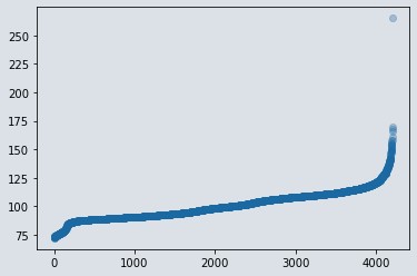
Figure 1 : Scatter plot of target variable
    # Distribution of target variable
    df[['y']].boxplot(figsize=(10,8))
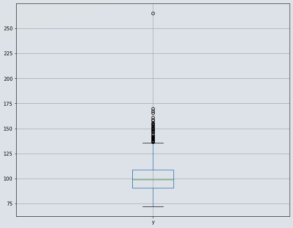
Figure 2 : Visualize distribution of target variable using boxplot
    # Have a look at the histogram to check for skewness
    df[['y']].hist(figsize=(10,8),bins=70)
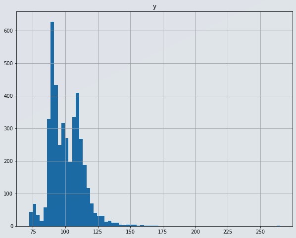
Figure 3 : Histogram of target variable
From above we conclude that,
- We have 4208 rows and 378 columns with 1 float that is target variable , 369 int with 0/1 values. Incidentally, this means those are also categorical variables and 8 object(categorical) values with multiple categories.
- Our target variable 'y' is not following normal distribution. Transorming target data to normal distribution will be the right approach in this case.
- We have detected one datapoint which is lying at 250 sec. even though it is valid but it is far away from all other datapoints so consider it as an outlier and we will remove that data row. If we don't do that, then it will affect our regression analysis.
    # remove instance/record with extreme value in target variable
    df = df[df.y < 225]

    # Visually check the target variable
    plt.scatter(range(len(df)), np.sort(df.y.values), alpha=0.3)
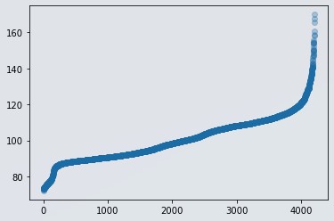
Figure 4 : Scatter plot of dependent variable without outlier data
Now we know that we have 378 columns in our dataset. Availability of more number of features may not help in getting generalised model, in data science world this situation is known as Curse of dimensionality. Just to make generalised model we should have to use dimensionality reduction technics and we can neglect the features having low variance this will help to get reduce the number of features that doesnt help in regression. Handling low variance features become very easy with pycaret just we have to set the option true. if you want to learn how to handle low variance features with pandas i will share the code at the end of the project. just look at there.
Lets Build Model using Pycaret
Pycaret is very simple and low code library though you should have knowledge about your dataset, what type of treatment you required. In above dataset exploration we found some interesting facts what we should have to do in preprocessing. Pycaret will build a pipeline for all those options which you turned on. As a ML Engineer you should know what you have to do with the dataset to get desired output right, otherwise it becomes garbage in garbage out type of situation. As our problem is of regression we will import regression from pycaret as below.
    from pycaret.regression import *

    # Lets verify our pycaret version as using same version only will reproduce same results
    pycaret.__version__
'2.3.0'
Generally we split the dataset into three parts, in 70:30:10 proportion for training, testing and validation purpose. Remember that train test split is also known as hold out method. Validation split dataset is the one which is unknown for model in its bulding and testing phase. This validation data split is used to validate the model metric accuracy, with metrics we got while building and testing. With pycaret, Hold out method or we say train test split is automatically done with setup, where we can specify propotions size too. If we want to change default train as 70% and test as 30%. we will split 10?ta for validation pupose as below.
    train_data = df.sample(frac=0.9, random_state=5)
    validation_data = df.drop(train_data.index)

    train_data.reset_index(drop=True, inplace=True)
    validation_data.reset_index(drop=True, inplace=True)

    print('Data for Modeling: ' + str(train_data.shape))
    print('Unseen Data For Predictions ' + str(validation_data.shape))
Data for Modeling: (3787, 378)
Unseen Data For Predictions (421, 378)
Very important part of pycaret library, is its setup. We will defining setup with utmost care as, what and how we feed decides what we get.
    reg = setup(data = train_data, target = 'y', train_size=0.8,
                ignore_features=['ID'], session_id=20,
                normalize=True, pca=True, pca_method='kernel',
                transform_target=True, ignore_low_variance = True,
                combine_rare_levels = True, remove_outliers=True)
Note:
Here we specified train size as 80% means test size will be 20% of train data. If we don't specify the train size, it will take train size as 70% by default.
- We have listed 'ID' feature in ignore features as ID is unique for each datapoint so it will add value in regression analysis.
- Session Id is just like random seed in sklearn used in order to control reproducibility so that every time whenever we run this code we get same result.
- normalize seting as true will use zscore method to standardize the data. Standardization is important so as to reduce bias error and reduce calculation time for some algorithms such as linear regression.
- PCA set as True will use dimensionality reduction technic PCA and setting PCA method as 'Kernel' will use PCA transformation using RVF kernel method. Here, with pycaret we do have three options for PCA method i.e linear, kernel and incremental (replacement of 'linear' when dataset is too large).
- transform taget set as true will transform target using box-cox method to help to build generalised ression model. Prediction results have usually improved after using this transformation.
- ignore_low_variance will ignore low variance features while building model. This will help to reduce dimensions and complexity of model by reducing those features which don't have much to add in model's predictive capability.
- combine_rare_levels set as true will combine the level which has very low appearance in dataset by combining that level with available categories in that column, which will help to reduce category levels. This in turn help's to reduce complexity of model.
- remove outliers set as true, will remove outliers considering datapoints which are far away from 95% of data. There is no need to mention missing values imputation, as by default pycaret will handle missing values smartly by imputing them automatically.
    # Lets verify available models list for regression
    models()
![]()
Figure 5 : Pycaret Model
Some models may not be seen in the output, just because in latest pycaret version you have to install those models such as catboost etc seperately..Post that it will be shown in your models section otherwise only default models will be used only..Also note, if you are using Google colab or binder or notebook then you will see these output or else you will have to manually check each object.
compare_model() function will compare all above models having turbo as true, if we want to exclude time consuming models then we can do it by specifying list of models to exclude parameter.
cm = compare_models(exclude = ['catboost','xgboost','lightgbm'], n_select=3)
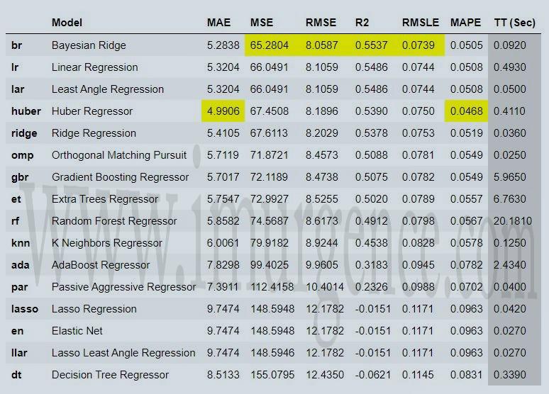
Figure 6 : Top3 performing model saved
we have mentioned n_select as 3 in compare model code and assigned it to cm variable. This will save top 3 performing models as a list in cm variable which we can use for further operations.
    # Lets verify what cm variable contains
    cm

[PowerTransformedTargetRegressor(alpha_1=1e-06, alpha_2=1e-06, alpha_init=None,
                                 compute_score=False, copy_X=True,
                                 fit_intercept=True, lambda_1=1e-06,
                                 lambda_2=1e-06, lambda_init=None, n_iter=300,
                                 normalize=False,
                                 power_transformer_method='box-cox',
                                 power_transformer_standardize=True,
                                 regressor=BayesianRidge(alpha_1=1e-06,
                                                         alpha_2=1e-06,
                                                         alpha_init=None,
                                                         compute_score=False,
                                                         copy_X=True,
                                                         fit_intercept=True,
                                                         lambda_1=1e-06,
                                                         lambda_2=1e-06,
                                                         lambda_init=None,
                                                         n_iter=300,
                                                         normalize=False,
                                                         tol=0.001,
                                                         verbose=False),
                                 tol=0.001, verbose=False),
 PowerTransformedTargetRegressor(copy_X=True, fit_intercept=True, n_jobs=-1,
                                 normalize=False,
                                 power_transformer_method='box-cox',
                                 power_transformer_standardize=True,
                                 regressor=LinearRegression(copy_X=True,
                                                            fit_intercept=True,
                                                            n_jobs=-1,
                                                            normalize=False)),
 PowerTransformedTargetRegressor(copy_X=True, eps=2.220446049250313e-16,
                                 fit_intercept=True, fit_path=True, jitter=None,
                                 n_nonzero_coefs=500, normalize=True,
                                 power_transformer_method='box-cox',
                                 power_transformer_standardize=True,
                                 precompute='auto', random_state=20,
                                 regressor=Lars(copy_X=True,
                                                eps=2.220446049250313e-16,
                                                fit_intercept=True,
                                                fit_path=True, jitter=None,
                                                n_nonzero_coefs=500,
                                                normalize=True,
                                                precompute='auto',
                                                random_state=20, verbose=False),
                                 verbose=False)]
We can use create model function when we are sure which model we want to use and don't want to waste our time in comparing all models.
    # For instance if we are sure to use svm
    svm_model = create_model('svm')
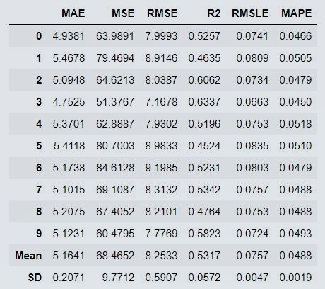
Figure 7 : SVM Model Performance Parameters ( If using Editors like Spyder, you may not get this output )
    predict_model(cm[0])
    # where cm[0] is first model(byesian regression) in cm variable list by using indexing we are using the same model for prediction.
    # In same way we an access second model i.e linear regression by using cm[1]
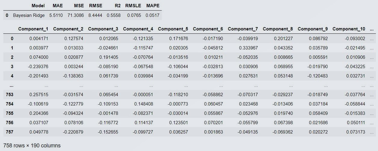
Figure 8 : Prediction on Test Data
Evaluate Model
evaluate_model(cm[0])
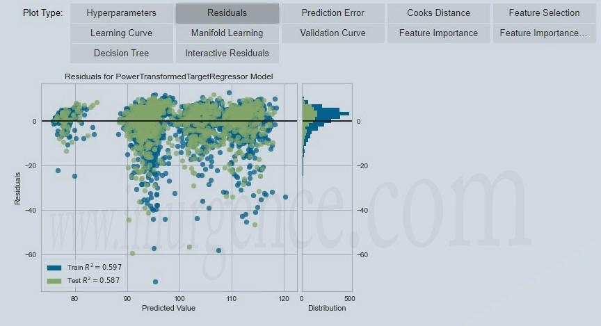
Figure 9 : Evaluate residuals
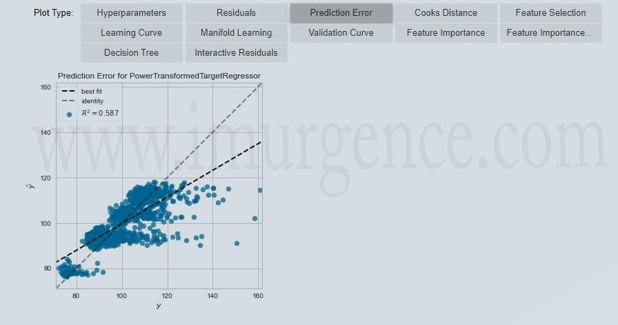
Figure 10 : Evaluate Prediction Errors
- Predicted model using test data which has been split during setup we can compare metrics if we found not much differnce in both train and predicted model metrics then its for sure our model is not overfitted. we can use the same model to predict target for new data after evaluation of plots.
- With evaluate_model() function we can evaluate model residuals plot, error plot, feature importance etc. This will help to decide whether to choose the model or not for deployment.
Stack Model
Stacking of models is also possible with pycaret in a very easy way. First of all we should know what stacking means..Stacking is the method in which all top models which we want to stack are treated as one model. Stacked model's predicted value is the averaage of each individual model's predicted value. Lets see how to stack the models
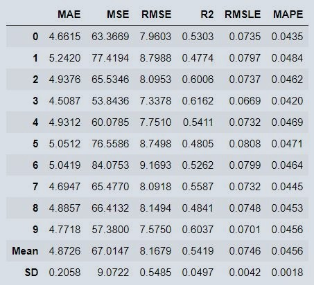
Figure 11 : Stacked Model Metrics
We can see a big difference in MAE metrics after stacking models. Individually we were geting MAE as approx 5.3, now its reduced to approx 4.9 with stacked model.
We will retest and predict the testing time on production line for test data
    # Lets check the test score
    predict_model(stacked)
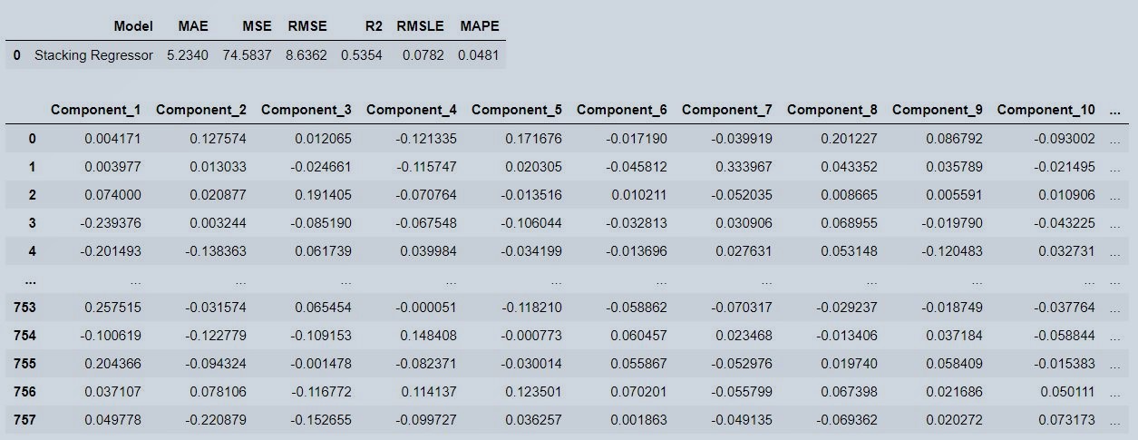
Figure 12 : Stacked Model Predictions
We are predicting the target variable i.e testing time on production line, from new unseen data by giving loaded model and validation data only to predict_model() function..thats it..
    new_prediction = predict_model(stacked,validation_data)
    new_prediction
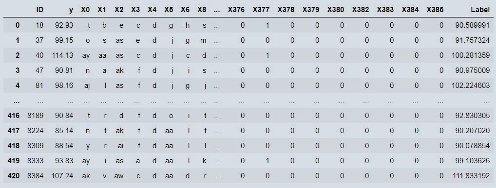
Figure 13 : Validation Data Output
    # Lets verify metrics of prediction on validation dataset.

    from pycaret.utils import check_metric
    newpredMAE = check_metric(new_prediction.y, new_prediction.Label, 'MAE')
    newpredMSE = check_metric(new_prediction.y, new_prediction.Label, 'MSE')
    newpredR2 = check_metric(new_prediction.y, new_prediction.Label, 'R2')

    print('New Prediction Metrics is as below: \n MAE = {}, \n MSE = {},\n R2 = {}'.format(newpredMAE,newpredMSE,newpredR2))
New Prediction Metrics is as below:
MAE = 5.131,
MSE = 68.0641,
R2 = 0.5641
Our validation score matches nearly to test score. Thus we can say its a generalised model.
Save Model for Reuse
save_model(stacked, 'stacked_model_time_prediction_mercedes_benze')
Transformation Pipeline and Model Succesfully Saved
(Pipeline(memory=None,
          steps=[('dtypes',
                  DataTypes_Auto_infer(categorical_features=[],
                                       display_types=False,
                                       features_todrop=['ID'], id_columns=[],
                                       ml_usecase='regression',
                                       numerical_features=[], target='y',
                                       time_features=[])),
                 ('imputer',
                  Simple_Imputer(categorical_strategy='not_available',
                                 fill_value_categorical=None,
                                 fill_value_numerical=None,
                                 numeric_strategy=...
                                                                                                eps=2.220446049250313e-16,
                                                                                                fit_intercept=True,
                                                                                                fit_path=True,
                                                                                                jitter=None,
                                                                                                n_nonzero_coefs=500,
                                                                                                normalize=True,
                                                                                                precompute='auto',
                                                                                                random_state=20,
                                                                                                verbose=False))],
                                                                              final_estimator=SVR(C=1.0,
                                                                                                  cache_size=200,
                                                                                                  coef0=0.0,
                                                                                                  degree=3,
                                                                                                  epsilon=0.1,
                                                                                                  gamma='scale',
                                                                                                  kernel='rbf',
                                                                                                  max_iter=-1,
                                                                                                  shrinking=True,
                                                                                                  tol=0.001,
                                                                                                  verbose=False),
                                                                              n_jobs=-1,
                                                                              passthrough=True,
                                                                              verbose=0),
                                                  verbose=0)]],
          verbose=False),
 'stacked_model_time_prediction_mercedes_benze.pkl')
    # Lets load the transformation pipeline and Model saved earlier for use
    stack = load_model('stacked_model_time_prediction_mercedes_benze')
With this we finished using Pycaret for predicting the "Testing time on Production Line" for the Mercedes-Benz dataset. Don't stop at this, although we had mentioned, ignore_low_variance = True, in the setup of pycaret , ideally we don't want this. Why don't you redo this who process by making sure that the zero variance variables are removed. To help you in this direction, we have compiled a small receipe, half cooked though so that you can explore and learn more.
First, find zero variance features is by calculating variance of features so that we can drop the features that contains zero variance. Note that, we are using full dataset here as we have to treat the whole dataset before any split.
    feature_data_var_df = pd.DataFrame(df.var(axis=0))
    feature_data_var_df[feature_data_var_df[0]==0]

    # lets define the list of columns to drop
    cols_to_drop = pd.Series.tolist(feature_data_var_df[feature_data_var_df[0]==0].index)

    # lets drop the columns not required from drop list
    df = df.drop(cols_to_drop,axis=1)
    print(df.shape)
Conclusion
We have build the project using advanced concepts of dimensionality reduction using PCA, handling low variance, combining rare levels categories, stacking of models in very easy way with the help of pycaret. If we have to do this with the help of sklearn only, then we might need lots of code to build the pipelines. We found that stacking of models helps to improve the metrics. Also our validation score matches with test scores pretty good, this is the indication that we have build a good generalized model. This is the real problem and real approach which we had covered in this project. Please do like and comment, if you find any issues in this project then please notify. Also, if you are just getting to learn pycaret then you should read this "Loan Approval Case Study in Python: A step by step guide on how to create a loan approval model in python using Pycaret"
About the Author:
Write A Public Review