Table of Content
Inspiration
Dataset exploration
Dependency Packages Installation in python
Loading Dataset
Loading Libraries
Basic EDA
Features Exploration
Lets Build Model using Pycaret
Conclusion
Inspiration
The object of this project is to identify which loan application needs to be approved or disapproved, in order to help the financial institutions like banks, NBFC's, etc take lending decisions at an operational level.
The banks or financial firms always have a risk while granting a loan to the loan applicant, who may not pay back and this is one of the reason for banks to accrue debt. Just imagine if we can build a model which can provide us with a risk or probability score to classify applicant as high or low default risk. In short we can approve/disapprove loan basis the risk score which reduces the financial risk.
This project is to build that predictive capability using machine learning algorithms. In this project we will explore low code pycaret library.
Dataset Exploration
We got some information about Loan Applicants in this dataset. We have total 13 independent variable, amongst them one is target variable.
Loan_ID: Its a unique ID assigned to every loan applicant
Gender: Male or Female
Married: The marital status of the applicant
Dependents: people dependent on the applicant (0,1,2,3+)
Education: Graduated or Not Graduated
Self_Employed: applicant is self-employed or not
ApplicantIncome: applicant earning income amount
CoapplicantIncome: co-applicant earning income amount
LoanAmount: The amount of loan the applicant has requested for
Loan_Amount_Term: The no. of days over which the loan will be paid
Credit_History: A record of a borrower's responsible repayment of debts, all debts paid or not
Property_Area: location where the applicant’s property lies Rural, Semiurban, Urban
Loan_Status: 1 for loan granted, 0 for not granted
Dependency Packages Installation in python
We are installing packages in python by using “pip” followed by install package name. For example, write “ !pip install pycaret ” and run that tab when you are using jupyter notebook. If you are using a editor you have to modify the script accordingly, for instance, if you are using the anaconda distribution then you can use navigator to install the package or you can use the anaconda prompt where you can type - "pip install pycaret" to install. Its better if you create a new environment in anaconda navigator or command prompt, wherein you use python 3.6 version. This would avoid disturbing your existing dependencies build for other projects.
Required packages for this project are as below:
Pandas - to perform dataframe operations
Numpy - to perform array operations
Matplotlib - to plot charts
Seaborn - to plot charts
Missingno - anlysing the missing values
pycaret - to build the model and save the model.
Loading Dataset
We have kept the data sets for building the model and testing in two separate files. Click on the links below to download the respective data sets.
Training Loan data set
Testing Loan data set
Loading Libraries
    import pandas as my_pd
    import numpy as my_np
    import missingno as my_msno
    import matplotlib.pyplot as my_plt
    import seaborn as my_sns

    # To enable plotting graphs in Jupyter notebook
    %matplotlib inline

    # Loading the dataset( note: data file must be in same directory)
    df_loan =my_pd.read_csv('data_loan_train.csv')
Basic EDA
We will verify whether our dataset is balanced or not. Balanced dataset is the one which has same amount of input data for every output classes. We will also check whether it contains outliers or not, how many missing values present in our dataset and so on..
    # Check dataset is Balanced dataset or not using frequency of target variable levels
    print(df_loan.Loan_Status.value_counts())

    # Visualize the frequency of target by class by plotting horizontal bar plot
    df_loan.Loan_Status.value_counts().plot(kind='barh')
Figure 1 : Target variable distribution using horizontal bar plot
We observe that the data is imbalanced.
    # Look at the statistical parameters of the data
    df_loan.describe()
Figure 2 : Statistical parameters of the data
We observe in figure 2 that LoanAmount, Loan_Amount_Term and Credit_History has less observation count as compared to other variables. The distribution of the features as well as the target variables are not uniform. We do have total dataset length as 491 where applicant income and co-applicant income both are highly skewed.
    # Check for Missing data
    df_loan.isnull().sum()
Figure 3 : Missing Data Count
    # Graphical representation of missing data
    my_msno.bar(df_loan, figsize=(8,6),fontsize=10)
Figure 4 : Missing data representation using missingno function
    # Box plot of the data set
    df_loan.boxplot(figsize=(20,8))
Figure 5 : Box plot of the data
From figure 5, we came to know that our dataset contains missing values and we do have outliers. We would have to impute missing values and remove the outliers. Don’t worry we will be using pycaret library to build the model and it will do these all things for us with just marking that option as True.
Features Exploration
    # Explore the features in the data using pair plot
    my_sns.pairplot(df_loan, hue='Loan_Status')
Figure 6 : Feature exploration using pair plot
From the pairplot in figure 6, it is clear that when credit history value is one, which means all debt repayment done, maximum loan application was granted, which makes sense too, right?. It means credit_history might be important predictor for us. All other predictors are not linearly separable. This takes me to take decision for building clusters while defining pycaret setup.
Lets Build Model using Pycaret
Use of pycaret is very simple as its low code library though you should have knowledge about your dataset, which type of treatment you need and so on. Pycaret will build a pipeline for all those options which you have turned on. As a ML Engineer you should know what you have to do with the dataset to get desired output right, otherwise it becomes garbage in garbage out type of situation.
As our problem is of classification we will import classification from pycaret as below
from pycaret.classification import *
Important part of pycaret library is its setup. We will be defining the setup with care as what and how we feed decides what we get.
    reg = setup(data=df_loan, target = 'Loan_Status',
                ignore_features=['Loan_ID'],
                train_size=0.80,
                remove_outliers=True,
                create_clusters=True,
                fix_imbalance=True,
                normalize=True,session_id=1975)    # session_id is equivalent to seed in randomization
we had defined reg variable for setup, just for reusing purpose of same setup. We ignore ‘Loan_ID’ feature as each applicant has a unique id and its of no use for building model, we have defined train size as 80% so it will automatically takes 20% for testing purpose.
We set outliers removal as True, thus it will automatically remove outliers which are more than 5% out of the normal data range (its the default setting we can change it also as per our requirement).
Fix_imbalance setting as True will balanced our dataset according to counts of Loan_status which is our output variable by using SMOTE.
Create clusters will add new feature to training dataset by clustering the dataset.
Normalize when set as true will standardize the dataset using standard scalar().
In short we define all preprocessing in pycaret setup.
There are lots of preprocessing options in pycaret setup, although we have to define requirement as per our dataset requirements
When we run this setup tab it will prompt a variable and datatype chart as pycaret automatically detects the datatype of variables we have to confirm the same, if found any issue then we will redefine setup and mention specific features type. Once we have done confirmation and pressed enter then it starts preparing preprocessing pipeline to use.
If you want you can check the content of reg, by using reg[0],reg[1], reg[2],.. and so on. Its a tuple of size 41.
Figure 7 : Compare output of various ML models
Here in figure 7, we compare various models with simple compare models code and assigned it to a variable which in turn saves best selected model which is highlighted by yellow color.
Next step is to compare the various models and their results so we using
cm= compare_models()
Lets verify what ‘cm’ variable contains.
cm
Figure 8 : Parameters of compare model object
Now, next step is to evaluate our model, evaluate_model() will give all available evaluation methods,graphs. We can plot it separately by using plot_model() as below,
plot_model(cm, plot = 'confusion_matrix')
Figure 9 : Plot of Confusion Matrix
We will predict the Loan_status of 20 % test data we separated in setup by using,
    prediction = predict_model(cm)
    prediction
Figure 10 : Prediction Snapshot
As we can see in figure 10, our preprocessed data cluster columns were added in the original data , ‘Label’ is the class prediction.
Our cross validated metrics from test and train data are not that much varying means our model is not over fitted nor under fitted as well.
We can separate out all three focus columns as below,
prediction[['Loan_Status','Label']]
Figure 11 : View focus columns
Now next step is to finalize the model in this way we will rebuild the same model on total data.
    # cm is variable assigned to best selected model
    final = finalize_model(cm)
Now we are ready with the model and can save it for reuse in future for new dataset.
save_model(final, 'loan_prediction')
Figure 12 : Snapshot of saved model
Now we can predict the loan status from new data whenever we want, lets see how to do that,
    # load the saved model
    model = load_model('loan_prediction')
After loading the model we have assigned it to a variable. After that we load our new data by using read_csv function.
df_loan_test = my_pd.read_csv('data_loan_test.csv')
Now we are just one step away from predicting loan status on new data. With a single line code pass the loaded model and dataset as input and run the tab ..boom ..job done.
predict_model(model, df_loan_test)
Figure 13 : View Final Prediction
Label is our prediction, 1 implies loan application should be approved and 0 implies loan application should not be approved.
Conclusion
We saw a simple way to create machine learning models using low code library. Almost every preprocessing becomes quite easy with pycaret and comparing models. There is much more advanced things also we can do with pycaret. Try the pycaret package for this other classification problem on Cancer data set. We will have a next tutorial blog with some advance technics and how they become very handy and easy to use with pycaret. Thanks for reading and be connected, please comment below your opinions.
About the Author:
Ganesh Kumar
Ganeshkumar Patel, is a Mechanical Engineer and applies data science for his process improvement. He loves to play with data and algorithms. During his spare time he likes to pen down his knowledge as a blogger.
Mohan Rai
Mohan Rai is an Alumni of IIM Bangalore , he has completed his MBA from University of Pune and Bachelor of Science (Statistics) from University of Pune. He is a Certified Data Scientist by EMC.Mohan is a learner and has been enriching his experience throughout his career by exposing himself to several opportunities in the capacity of an Advisor, Consultant and a Business Owner. He has more than 18 years’ experience in the field of Analytics and has worked as an Analytics SME on domains ranging from IT, Banking, Construction, Real Estate, Automobile, Component Manufacturing and Retail. His functional scope covers areas including Training, Research, Sales, Market Research, Sales Planning, and Market Strategy.
Table of Content
- Inspiration
- Dataset exploration
- Dependency Packages Installation in python
- Loading Dataset
- Loading Libraries
- Basic EDA
- Features Exploration
- Lets Build Model using Pycaret
- Conclusion
The object of this project is to identify which loan application needs to be approved or disapproved, in order to help the financial institutions like banks, NBFC's, etc take lending decisions at an operational level.
The banks or financial firms always have a risk while granting a loan to the loan applicant, who may not pay back and this is one of the reason for banks to accrue debt. Just imagine if we can build a model which can provide us with a risk or probability score to classify applicant as high or low default risk. In short we can approve/disapprove loan basis the risk score which reduces the financial risk.
This project is to build that predictive capability using machine learning algorithms. In this project we will explore low code pycaret library.
We got some information about Loan Applicants in this dataset. We have total 13 independent variable, amongst them one is target variable.
- Loan_ID: Its a unique ID assigned to every loan applicant
- Gender: Male or Female
- Married: The marital status of the applicant
- Dependents: people dependent on the applicant (0,1,2,3+)
- Education: Graduated or Not Graduated
- Self_Employed: applicant is self-employed or not
- ApplicantIncome: applicant earning income amount
- CoapplicantIncome: co-applicant earning income amount
- LoanAmount: The amount of loan the applicant has requested for
- Loan_Amount_Term: The no. of days over which the loan will be paid
- Credit_History: A record of a borrower's responsible repayment of debts, all debts paid or not
- Property_Area: location where the applicant’s property lies Rural, Semiurban, Urban
- Loan_Status: 1 for loan granted, 0 for not granted
We are installing packages in python by using “pip” followed by install package name. For example, write “ !pip install pycaret ” and run that tab when you are using jupyter notebook. If you are using a editor you have to modify the script accordingly, for instance, if you are using the anaconda distribution then you can use navigator to install the package or you can use the anaconda prompt where you can type - "pip install pycaret" to install. Its better if you create a new environment in anaconda navigator or command prompt, wherein you use python 3.6 version. This would avoid disturbing your existing dependencies build for other projects.
Required packages for this project are as below:
- Pandas - to perform dataframe operations
- Numpy - to perform array operations
- Matplotlib - to plot charts
- Seaborn - to plot charts
- Missingno - anlysing the missing values
- pycaret - to build the model and save the model.
We have kept the data sets for building the model and testing in two separate files. Click on the links below to download the respective data sets.
Training Loan data set
Testing Loan data set
import pandas as my_pd
import numpy as my_np
import missingno as my_msno
import matplotlib.pyplot as my_plt
import seaborn as my_sns
# To enable plotting graphs in Jupyter notebook
%matplotlib inline
# Loading the dataset( note: data file must be in same directory)
df_loan =my_pd.read_csv('data_loan_train.csv')
We will verify whether our dataset is balanced or not. Balanced dataset is the one which has same amount of input data for every output classes. We will also check whether it contains outliers or not, how many missing values present in our dataset and so on..
# Check dataset is Balanced dataset or not using frequency of target variable levels
print(df_loan.Loan_Status.value_counts())
# Visualize the frequency of target by class by plotting horizontal bar plot
df_loan.Loan_Status.value_counts().plot(kind='barh')
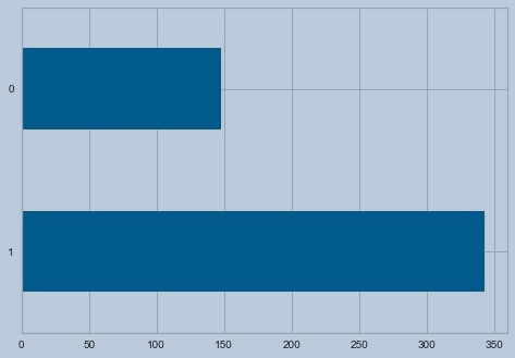
Figure 1 : Target variable distribution using horizontal bar plot
We observe that the data is imbalanced.
# Look at the statistical parameters of the data
df_loan.describe()
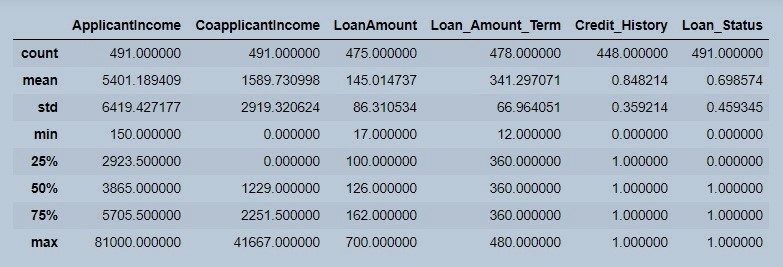
Figure 2 : Statistical parameters of the data
We observe in figure 2 that LoanAmount, Loan_Amount_Term and Credit_History has less observation count as compared to other variables. The distribution of the features as well as the target variables are not uniform. We do have total dataset length as 491 where applicant income and co-applicant income both are highly skewed.
# Check for Missing data
df_loan.isnull().sum()
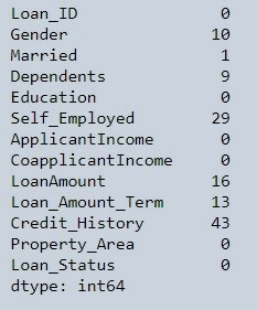
Figure 3 : Missing Data Count
# Graphical representation of missing data
my_msno.bar(df_loan, figsize=(8,6),fontsize=10)
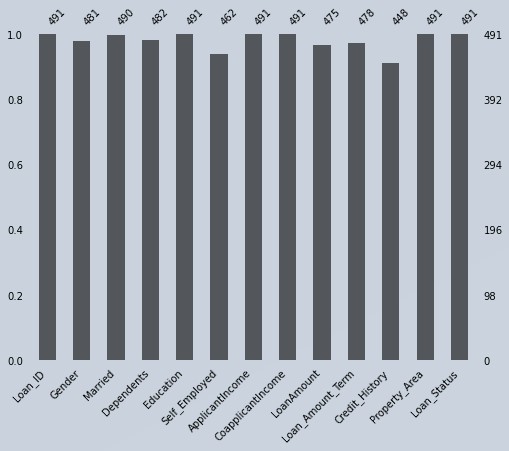
Figure 4 : Missing data representation using missingno function
# Box plot of the data set
df_loan.boxplot(figsize=(20,8))
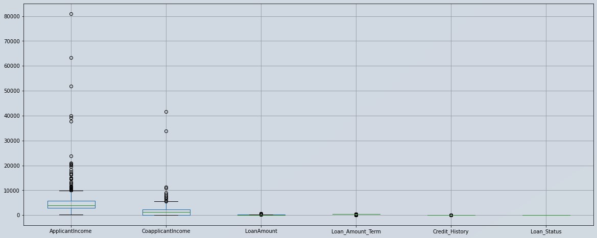
Figure 5 : Box plot of the data
From figure 5, we came to know that our dataset contains missing values and we do have outliers. We would have to impute missing values and remove the outliers. Don’t worry we will be using pycaret library to build the model and it will do these all things for us with just marking that option as True.
# Explore the features in the data using pair plot
my_sns.pairplot(df_loan, hue='Loan_Status')
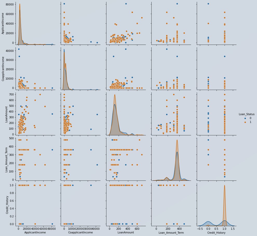
Figure 6 : Feature exploration using pair plot
From the pairplot in figure 6, it is clear that when credit history value is one, which means all debt repayment done, maximum loan application was granted, which makes sense too, right?. It means credit_history might be important predictor for us. All other predictors are not linearly separable. This takes me to take decision for building clusters while defining pycaret setup.
Use of pycaret is very simple as its low code library though you should have knowledge about your dataset, which type of treatment you need and so on. Pycaret will build a pipeline for all those options which you have turned on. As a ML Engineer you should know what you have to do with the dataset to get desired output right, otherwise it becomes garbage in garbage out type of situation.
As our problem is of classification we will import classification from pycaret as below
from pycaret.classification import *
Important part of pycaret library is its setup. We will be defining the setup with care as what and how we feed decides what we get.
reg = setup(data=df_loan, target = 'Loan_Status',
ignore_features=['Loan_ID'],
train_size=0.80,
remove_outliers=True,
create_clusters=True,
fix_imbalance=True,
normalize=True,session_id=1975) # session_id is equivalent to seed in randomization
we had defined reg variable for setup, just for reusing purpose of same setup. We ignore ‘Loan_ID’ feature as each applicant has a unique id and its of no use for building model, we have defined train size as 80% so it will automatically takes 20% for testing purpose.
We set outliers removal as True, thus it will automatically remove outliers which are more than 5% out of the normal data range (its the default setting we can change it also as per our requirement).
Fix_imbalance setting as True will balanced our dataset according to counts of Loan_status which is our output variable by using SMOTE.
Create clusters will add new feature to training dataset by clustering the dataset.
Normalize when set as true will standardize the dataset using standard scalar().
In short we define all preprocessing in pycaret setup.
There are lots of preprocessing options in pycaret setup, although we have to define requirement as per our dataset requirements
When we run this setup tab it will prompt a variable and datatype chart as pycaret automatically detects the datatype of variables we have to confirm the same, if found any issue then we will redefine setup and mention specific features type. Once we have done confirmation and pressed enter then it starts preparing preprocessing pipeline to use.
If you want you can check the content of reg, by using reg[0],reg[1], reg[2],.. and so on. Its a tuple of size 41.
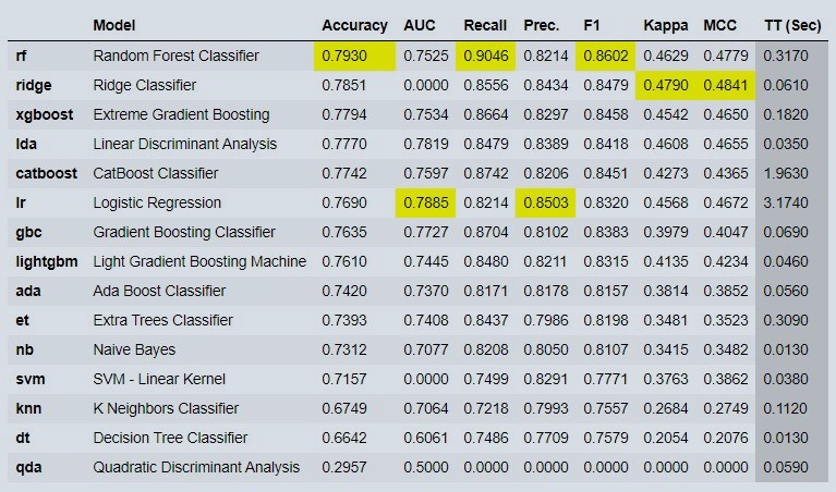
Figure 7 : Compare output of various ML models
Here in figure 7, we compare various models with simple compare models code and assigned it to a variable which in turn saves best selected model which is highlighted by yellow color.
Next step is to compare the various models and their results so we using
cm= compare_models()
Lets verify what ‘cm’ variable contains.
cm
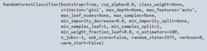
Figure 8 : Parameters of compare model object
Now, next step is to evaluate our model, evaluate_model() will give all available evaluation methods,graphs. We can plot it separately by using plot_model() as below,
plot_model(cm, plot = 'confusion_matrix')
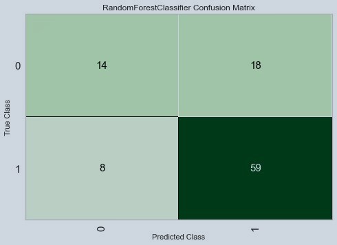
Figure 9 : Plot of Confusion Matrix
We will predict the Loan_status of 20 % test data we separated in setup by using,
prediction = predict_model(cm)
prediction
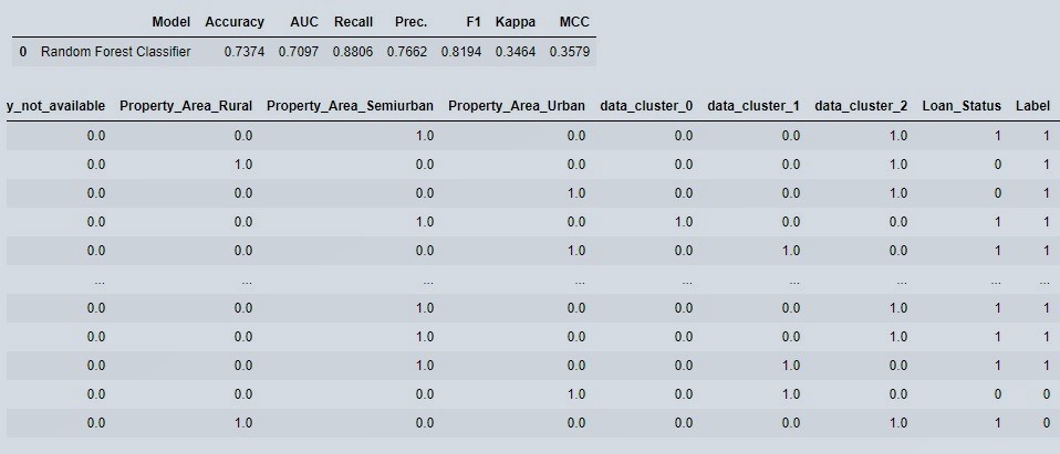
Figure 10 : Prediction Snapshot
As we can see in figure 10, our preprocessed data cluster columns were added in the original data , ‘Label’ is the class prediction.
Our cross validated metrics from test and train data are not that much varying means our model is not over fitted nor under fitted as well.
We can separate out all three focus columns as below,
prediction[['Loan_Status','Label']]
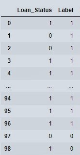
Figure 11 : View focus columns
Now next step is to finalize the model in this way we will rebuild the same model on total data.
# cm is variable assigned to best selected model
final = finalize_model(cm)
Now we are ready with the model and can save it for reuse in future for new dataset.
save_model(final, 'loan_prediction')
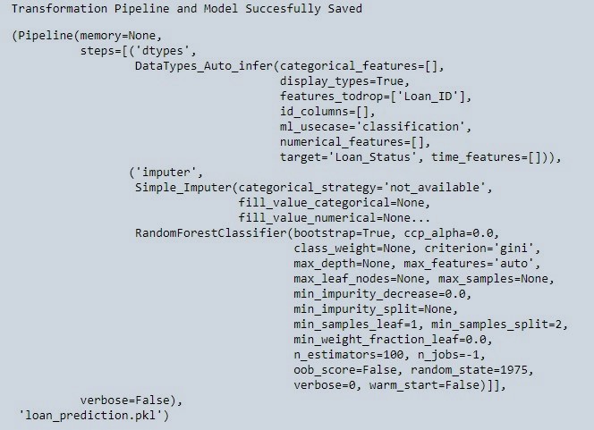
Figure 12 : Snapshot of saved model
Now we can predict the loan status from new data whenever we want, lets see how to do that,
# load the saved model
model = load_model('loan_prediction')
After loading the model we have assigned it to a variable. After that we load our new data by using read_csv function.
df_loan_test = my_pd.read_csv('data_loan_test.csv')
Now we are just one step away from predicting loan status on new data. With a single line code pass the loaded model and dataset as input and run the tab ..boom ..job done.
predict_model(model, df_loan_test)
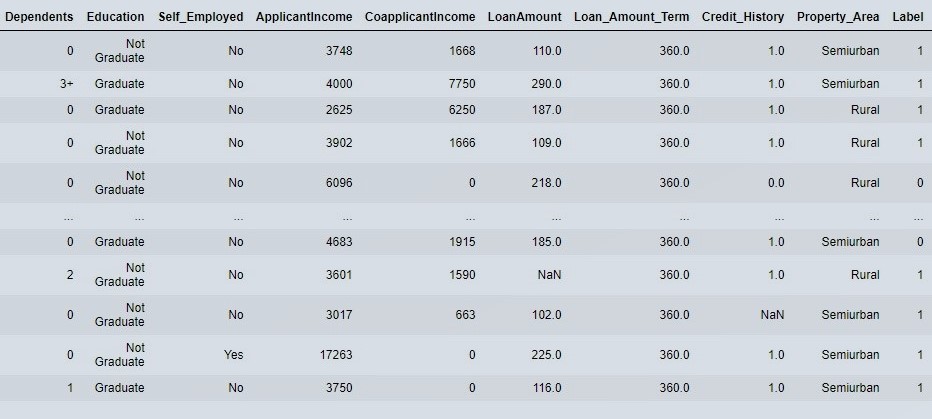
Figure 13 : View Final Prediction
Label is our prediction, 1 implies loan application should be approved and 0 implies loan application should not be approved.
We saw a simple way to create machine learning models using low code library. Almost every preprocessing becomes quite easy with pycaret and comparing models. There is much more advanced things also we can do with pycaret. Try the pycaret package for this other classification problem on Cancer data set. We will have a next tutorial blog with some advance technics and how they become very handy and easy to use with pycaret. Thanks for reading and be connected, please comment below your opinions.
About the Author:

Write A Public Review