
Table of Contents
- Machine Learning in Medical Insurance
- About the Data
- Importing required Libraries
- Importing Dataset
- Data Analysis
- Data Pre – Processing
- Splitting the Features and Target
- Splitting Dataset into Training data & Testing data
- Model Selection & Model Training
- Model Evaluation
- Building a Predictive System
- Conclusion
About Medical Insurance
Before creating Medical Insurance Cost Prediction model, Let’s understand what is Medical Insurance and how it can help us. Medical Insurance is a type of Insurance that covers yours medical expenses that arise due to an illness. These can be related to medicine cost, Doctor consultation fee, procedures or hospitalization cost etc.
Machine Learning in Medical Insurance
In this we will discuss about the Problem Statement of our Project it says that :- An Insurance Company wants to predict medical insurance cost of a person using Machine Learning by providing relevant data.
That cost predicted by our machine learning model will be suggested to their customer who wants to buy a medical insurance from that company. In developed economies there are various stakeholders, namely buyer, insurer and health care service provider. The objectives of all the stake holders are different. A lot of automation using ML is implemented these days, for instance AI based appointment voice BOT is used to reduce call abandonment rate. We would cover this implementation in some other project. For now lets focus on the Insurance cost assessment.
Importing required Libraries
    import numpy as np
    import pandas as pd
    import matplotlib.pyplot as plt
    import seaborn as sns
    from sklearn.model_selection import train_test_split
    from xgboost import XGBRegressor
    from sklearn import metrics
    import warnings
    warnings.filterwarnings('ignore')
About the Data
Let’s explore the data. In this dataset there are some details like Age, Sex, BMI, Children, Smoker, Region and Charges. Download the data by clicking on this link, Medical Insurance Data.
Importing Dataset
    df = pd.read_csv("medical-insurance-data.csv")

    # first 5 rows of the dataframe
    df.head()

   age     sex     bmi  children smoker     region      charges
0   19  female  27.900         0    yes  southwest  16884.92400
1   18    male  33.770         1     no  southeast   1725.55230
2   28    male  33.000         3     no  southeast   4449.46200
3   33    male  22.705         0     no  northwest  21984.47061
4   32    male  28.880         0     no  northwest   3866.85520


    # number of rows and column
    df.shape
(1338, 7)

    # getting some informations about the dataset
    df.info()


RangeIndex: 1338 entries, 0 to 1337
Data columns (total 7 columns):
 #   Column    Non-Null Count  Dtype
---  ------    --------------  -----
 0   age       1338 non-null   int64
 1   sex       1338 non-null   object
 2   bmi       1338 non-null   float64
 3   children  1338 non-null   int64
 4   smoker    1338 non-null   object
 5   region    1338 non-null   object
 6   charges   1338 non-null   float64
dtypes: float64(2), int64(2), object(3)
memory usage: 73.3+ KB
There are no null values in the dataset
Data Analysis
    # Statistical Measures of the dataset
    df.describe()

               age          bmi     children       charges
count  1338.000000  1338.000000  1338.000000   1338.000000
mean     39.207025    30.663397     1.094918  13270.422265
std      14.049960     6.098187     1.205493  12110.011237
min      18.000000    15.960000     0.000000   1121.873900
25 per     .000000    26.296250     0.000000   4740.287150
50 per    9.000000    30.400000     1.000000   9382.033000
75 per     .000000    34.693750     2.000000  16639.912515
max      64.000000    53.130000     5.000000  63770.428010
    # distribution of age value
    sns.set()
    plt.figure(figsize=(8,6))
    sns.distplot(df['age'])
    plt.title('Age Distribution')
    plt.show()
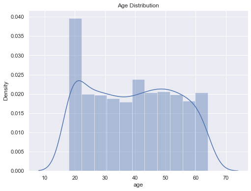
Figure 1 : Plot of Age Distribution
    # Gender column
    plt.figure(figsize=(7,6))
    sns.countplot(x = 'sex', data = df)
    plt.title('Gender Distribution', fontsize = 15, fontweight = 'bold')
    plt.show()
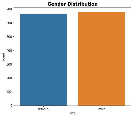
Figure 2 : Plot of Gender Distribution
    df['sex'].value_counts()

male      676
female    662
Name: sex, dtype: int64
    # bmi distribution
    plt.figure(figsize=(8,6))
    sns.distplot(df['bmi'])
    plt.title('BMI Distribution', fontsize = 15, fontweight = 'bold')
    plt.show()
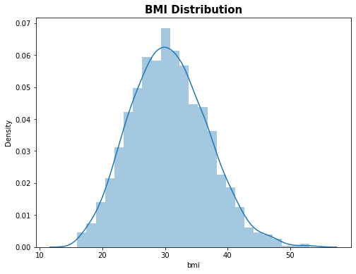
Figure 3 : Plot of BMI Distribution
    # children column
    plt.figure(figsize=(6,6))
    sns.countplot(x = 'children', data = df)
    plt.title('Children', fontsize = 15, fontweight = 'bold')
    plt.show()
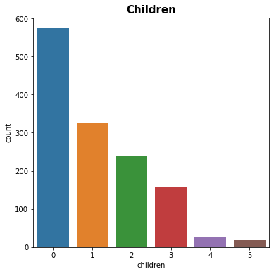
Figure 4 : Plot of Children Distribution
    df['children'].value_counts()

0    574
1    324
2    240
3    157
4     25
5     18
Name: children, dtype: int64
    # smoker column
    plt.figure(figsize=(6,6))
    sns.countplot(x = 'smoker', data = df)
    plt.title('Smoker', fontsize = 15, fontweight = 'bold')
    plt.show()
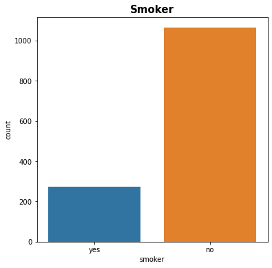
Figure 5 : Plot of Smoker Distribution
    df['smoker'].value_counts()

no     1064
yes     274
Name: smoker, dtype: int64
    # region column
    plt.figure(figsize=(6,6))
    sns.countplot(x = 'region', data = df)
    plt.title('Region', fontsize = 15, fontweight = 'bold')
    plt.show()
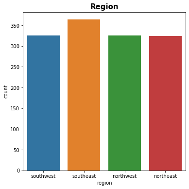
Figure 6 : Plot of Region Distribution
    df['region'].value_counts()

southeast    364
northwest    325
southwest    325
northeast    324
Name: region, dtype: int64
    # distribution of charges value
    plt.figure(figsize=(8,6))
    sns.distplot(df['charges'])
    plt.title('Charges Distribution', fontsize = 15, fontweight = 'bold')
    plt.show()
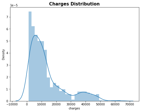
Figure 7 : Plot of Charges Distribution
Data Pre-Processing
Encoding the categorical features
Replace male & female with 0 & 1 respectively. Replace yes & no in smoker with 0 and 1 respectively. Replace southeast, southwest, northeast and northwest with 0, 1, 2, 3 respectively.
    # replacing male & female column with 0 & 1 respectively
    df.replace({'sex':{'male':0,'female':1}}, inplace=True)

    # replacing smoker yes & no column with 0 & 1 respectively
    df.replace({'smoker':{'yes':0,'no':1}}, inplace=True)

    # replacing southeast, southwest, northeast, northwest column with 0, 1, 2, 3 respectively
    df.replace({'region':{'southeast' :0,'southwest':1,'northeast':2,'northwest':3}}, inplace= True)
Splitting the Features and Target
    X = df.drop(columns='charges', axis = 1)
    y = df['charges']

    print(X)

      age  sex     bmi  children  smoker  region
0      19    1  27.900         0       0       1
1      18    0  33.770         1       1       0
2      28    0  33.000         3       1       0
3      33    0  22.705         0       1       3
4      32    0  28.880         0       1       3
      ...  ...     ...       ...     ...     ...
1333   50    0  30.970         3       1       3
1334   18    1  31.920         0       1       2
1335   18    1  36.850         0       1       0
1336   21    1  25.800         0       1       1
1337   61    1  29.070         0       0       3

[1338 rows x 6 columns]

    print(y)

0       16884.92400
1        1725.55230
2        4449.46200
3       21984.47061
4        3866.85520
                ...
1333    10600.54830
1334     2205.98080
1335     1629.83350
1336     2007.94500
1337    29141.36030
Name: charges, Length: 1338, dtype: float64
Splitting the dataset into Training Data & Testing Data
    X_train, X_test, y_train, y_test = train_test_split(X, y, test_size = 0.2, random_state = 2)
    print(X_train.shape)
    print(X_test.shape)
    print(y_train.shape)
    print(y_test.shape)

(1070, 6)
(268, 6)
(1070,)
(268,)
Model Training
XGBoost Regressor
    # loading the model
    model = XGBRegressor()
    # training the model with X_train, y_train
    model.fit(X_train, y_train)

XGBRegressor(base_score=0.5, booster='gbtree', colsample_bylevel=1,
             colsample_bynode=1, colsample_bytree=1, gamma=0, gpu_id=-1,
             importance_type='gain', interaction_constraints='',
             learning_rate=0.300000012, max_delta_step=0, max_depth=6,
             min_child_weight=1, missing=nan, monotone_constraints='()',
             n_estimators=100, n_jobs=4, num_parallel_tree=1, random_state=0,
             reg_alpha=0, reg_lambda=1, scale_pos_weight=1, subsample=1,
             tree_method='exact', validate_parameters=1, verbosity=None)
Model Evaluation
    train_data_prediction = model.predict(X_train)
    print(train_data_prediction)

[ 2322.9866  6243.888  11853.557  ... 12549.385  10701.751  12098.009 ]

    # Getting R squared value for training dataset
    r2_train = metrics.r2_score(y_train, train_data_prediction)
    print('R squared value for training dataset : ', r2_train)

R squared value for training dataset :  0.9962665931681515
R square value lies in range of 0 to 1. The more it is closer to 1 , more the model will perform well.
    test_data_prediction = model.predict(X_test)
    # R squared value for testing dataset

    r2_train = metrics.r2_score(y_test, test_data_prediction)
    print('R squared value for testing dataset : ', r2_train)

R squared value for testing dataset :  0.8217591365018906
Building a Predictive system
    # Replace male & female with 0 & 1 respectively.
    # Replace yes & no in smoker with 0 and 1 respectively.
    # Replace southeast, southwest, northeast and northwest with 0, 1, 2, 3 respectively.

    input_data = (21,1,16.815,1,1,2)

    # changing input_data to a numpy array
    input_data_as_numpy_array = np.asarray(input_data)

    # reshape the array
    input_data_reshaped = input_data_as_numpy_array.reshape(1,-1)

    prediction = model.predict(input_data_reshaped)

    print('The insurance cost is', prediction[0])

The insurance cost is 3166.413
Conclusion
Here above we have successfully build a Machine Learning model using XGBoost Regressor and predicted the cost of Insurance. But, before that we have collected
- The data
- Imported necessary libraries
- Performed data pre – processing
- Analyzed data Visually
- Split the data into training and testing data
- Selecting and Training Model
- Performed Model Evaluation.
- And at last we build a predictive system.
You can add more layers to this for optimizing your model, for instance you can use cross validation's to generalize the model. Have a look at this application of Cross Validation.
About the Author's:
Write A Public Review