How to do Object Detection in Python Using YOLO ?
Introduction
YOLO = you only look once
Yolo is a method for detecting objects. It is the quickest method of detecting objects.
In the field of computer vision, it's also known as the standard method of object detection.
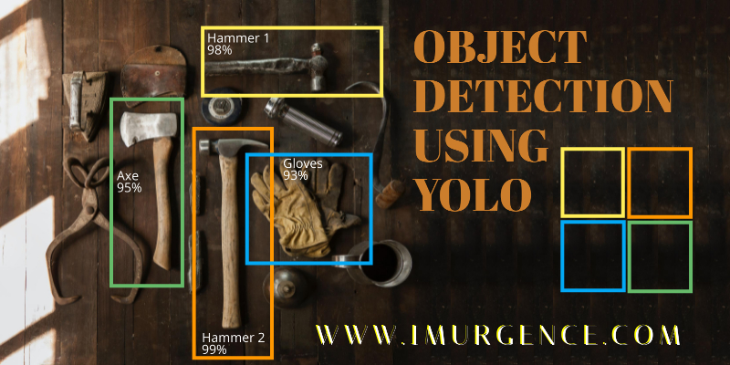
Between 2015 and 2016, Yolo gained popularity. Before 2015, People used to use algorithms like the sliding window object detection algorithm, but then R CNN, Fast R CNN, and Faster R CNN became popular. We don't simply detect photos in Yolo. We also provide bounding boxes around the objects.
It was created by Joseph Redmon et al., and the initial version of Yolo was launched in 2016, followed by Yolo version 2 in 2017.Yolo v4 was published in 2020 after the third version was released in 2018. And recently Yolo version 5 has been released.
In the present execution, we are going to use yolov3, not the latest update yolov4 because yolov4 came with two weights files where the author didn't explain why the two weights have been used. And also Joseph Redmon was not the author anymore for Yolo v4 and v5, where it affects the Yolo algorithms and side deviation of many programmers and experts sharing their view as Yolo v3 recall speed is faster than the latest versions.
About Yolo and how it works.
YOLO is a real-time object identification Convolutional Neural Network (CNN). The program separates the image into areas and predicts bounding boxes and probabilities for each region using a single neural network. The projected probabilities are used to weigh the bounding boxes.
YOLO is popular because it has a high level of accuracy and can run in real-time. The approach takes only one forward propagation to run through the neural network to make predictions, so it "only looks once" at the image.
It then returns detected items together with bounding boxes after non-max suppression (which ensures that the object detection algorithm only discovers each object once).
Yolo emits a vector whenever it detects an object in an image. The vector holds all the information about the image that was found.
the vector consist of:-
P(object)*IOU(Intersection over union)
Bx
By
Bw
Bh
c1
c2
....
P(Object)*IOU
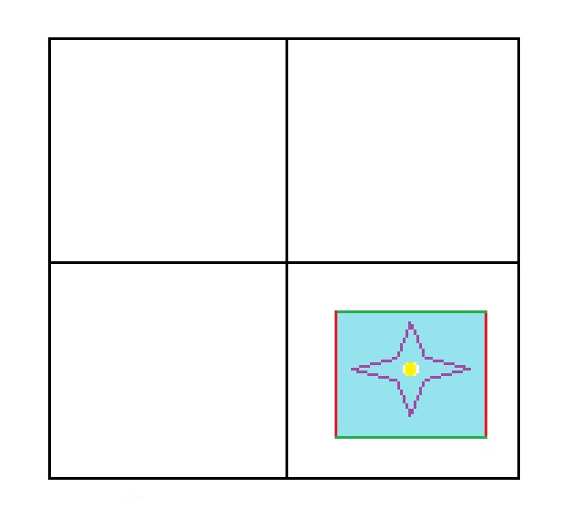
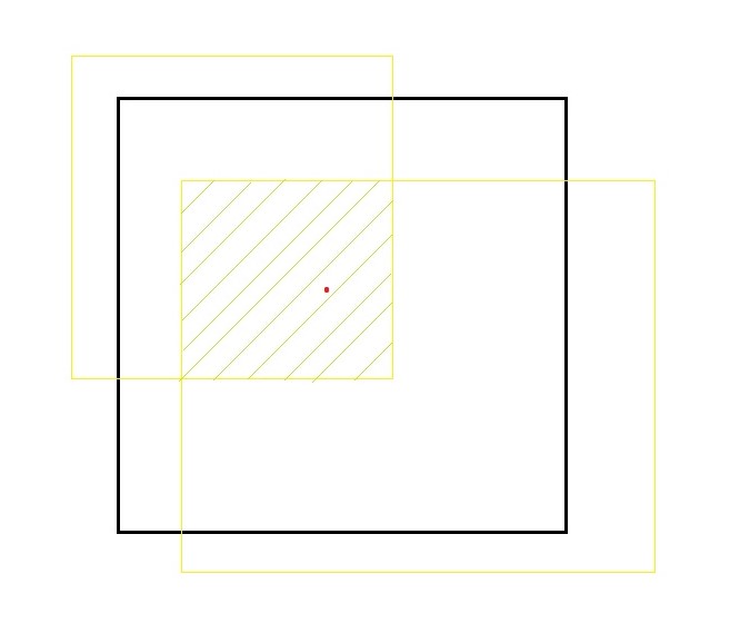
P(object)*IOU is known to be a confidence score. IOU is one of the most Important properties in Yolo.
The red colored dot is the center of the object identified. Where the black box is the bounded box (predicted box) and the yellow boxes are ground truth regions. We go with equation
IOU= Area of the intersection of all boxes/Area of the union of all boxes.
P(object)*IOU is required to be high because the high score indicates high accuracy.
Bx, By
The coordinates of the object's Centre are x and y.
Bw, Bh
w and h are the width and height (respectively) of the box bounded.
C1, C2, C3,...
These C's denotes all the classes in the model. When the object is identified to respective class it is numbered 1 and all the rest are denoted with 0(zero)
For example:
If we go through a scenario. Yolo with two classes (c1=dog and c2=cat), where an image with a cat is passed to the algorithm, we can expect the output vector as
{1,86,49,45,36,0,1}= {p(c),x,y,w,h,c1,c2} .
In the same scenario, if the image with the dog is passed then the output can be expected as
{1,86,49,34,36,1,0}={p(c),x,y,w,h,c1,c2}.
If the images with no objects is given then the output will be mostly
{0,0,0,0,0,0,0}={p(c),x,y,w,h,c1,c2}.
Always the p(c) will be somewhere between 0 and 1.
CODE
Importing all the requirements.
Weights and Cfg are the output files of the darknet detect train model. We also add classes to the program from the class file. Download this zip file , yolo-project.zip. This has all the pre requisites for executing the project, including the sample image files. You can unzip these files on to your working directory.
Implementation
    # Install below libraries using terminal
    # pip install pillow
    # pip install opencv-python

    # Importing libraries  into the project
    from PIL import Image
    import numpy as np
    import cv2
    # Resizing the image using pillow
    #image resize automation
    image = Image.open('yolo-test-image1.jpg')
    div=image.size[0]/500
    resized_image = image.resize((round(image.size[0]/div),round(image.size[1]/div)))
    resized_image.save('na.jpg')
    #yolov3 algoritham
    #importing weights
    classes_names=['person','bicycle','car','motorbike','aeroplane','bus','train','truck','boat','traffic light','fire hydrant','stop sign','parking meter','bench','bird','cat','dog','horse','sheep','cow','elephant','bear','zebra','giraffe','backpack','umbrella','handbag','tie','suitcase','frisbee','skis','snowboard','sports ball','kite','baseball bat','baseball glove','skateboard','surfboard','tennis racket','bottle','wine glass','cup','fork','knife','spoon','bowl','banana','apple','sandwich','orange','broccoli','carrot','hot dog','pizza','donut','cake','chair','sofa','pottedplant','bed','diningtable','toilet','tvmonitor','laptop','mouse','remote','keyboard','cell phone','microwave','oven','toaster','sink','refrigerator','book','clock','vase','scissors','teddy bear','hair drier','toothbrush']
    model=cv2.dnn.readNet("yolov3.weights","yolov3.cfg")
    layer_names = model.getLayerNames()
    output_layers=[layer_names[i[0]-1]for i in model.getUnconnectedOutLayers()]

    # Here we need to import the image which is previously resized for the neural network.
    image=cv2.imread("na.jpg")
    height, width, channels = image.shape
    # In the call to ,cv2.dnn.blobFromImage(image, scalefactor=1.0, size, mean, swapRB=True),size can be 224,224 for low quality 416,416 for medium quality.
Remember that we won't immediately use the entire image on the network; we'll need to convert it to a blob first. A Blob is a tool for extracting and resizing image features. The ideal scale factor for blob is 0.00392. Then there are many sizes for blob (224,224)(416,416) low and high sizes, respectively. Finally, the mean will be the RGB values we would like to pass to our Convolutional Neural Networks.
    blob=cv2.dnn.blobFromImage(image, 0.00392, (416,416), (0,0,0), True, crop=False)
    model.setInput(blob)
    outputs= model.forward(output_layers)
    class_ids = []
    confidences = []
    boxes = []
The detection is complete at this stage, and all that remains is to display the results on the screen. We then iterate through the outs array, calculating confidence and selecting a confidence threshold.
    for output in outputs:
        for identi in output:
            scores = identi[5:]
            class_id = np.argmax(scores)
            confidence = scores[class_id]
            if confidence > 0.8:
                # Object detected
                centerx = int(identi[0] * width)
                centery = int(identi[1] * height)
                w = int(identi[2] * width)
                h = int(identi[3] * height)
                # Rectangle coordinates
                x = int(centerx - w / 2)
                y = int(centery - h / 2)
                boxes.append([x, y, w, h])
                confidences.append(float(confidence))
                class_ids.append(class_id)
When performing the detection, we may find that we have multiple boxes for the same object, in which case we should use a different algorithm to remove this "noise."It's referred to as non-maximum suppression. cv2.dnn.NMSBoxes(boxes, confidences, SCORE_THRESHOLD, IOU_THRESHOLD) SCORE_THRESHOLD: The model is assumed to never return predictions with a score lower than this value. IOU_THRESHOLD: This value is used in object detection to calculate the overlap of an object's predicted and actual bounding boxes.
    indexes = cv2.dnn.NMSBoxes(boxes, confidences, 0.5, 0.4)
    font = cv2.FONT_HERSHEY_COMPLEX
    colors = np.random.uniform(0, 255, size=(len(classes_names), 3))
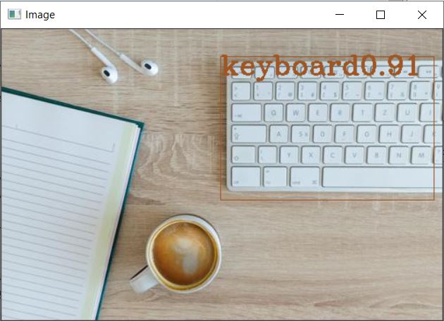
Finally, we place data on the image and display it. Using all the data we collected in the process. We place boxes and class names. We are placing a confidence score on the top of the box to show how accurate our model is in detecting objects.
    for i in range(len(boxes)):
        if i in indexes:
            x, y, w, h = boxes[i]
            confidence = str("{:.2f}".format(confidences[i]))
            label = str(classes_names[class_ids[i]]+confidence)
            color = colors[i]

            cv2.rectangle(image, (x, y), (x + w, y + h), color, 1)
            cv2.putText(image, label,(x, y + 20), font, 1, color, 2)

    cv2.imshow("Image",image)
    cv2.waitKey(0)
    cv2.destroyAllWindows()
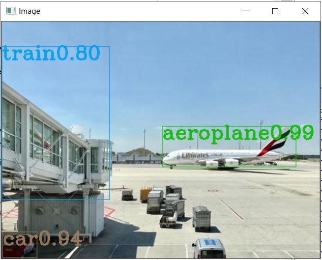
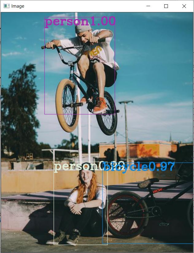
This is the Object identification observed on the first sample file. We need to iteratively run the code for the next three images as provided in the sample zip folder, or alternatively you can pack the whole code into a function and call it. Displayed herein is the result observed for the remaining three files as well.
Conclusion
In the above discussion, we have learned the working principle behind the Yolo algorithm and implementing it in python using OpenCV. However, with the help of the Yolo algorithm, we can detect objects in the real world with minimal time. Moreover, we can implement the Yolo algorithm on both images and videos. You can read more about object detection and human pose estimation in python using OpenCV.
About the Author's:
Sujith Kumar
Sujith Kumar is a Data Science intern at simple and real Analytics. He is a self-learning data science aspirant. Pursuing graduation bachelors in computer science and engineering at IIIT-RGUKT.
Mohan Rai
Mohan Rai is an Alumni of IIM Bangalore , he has completed his MBA from University of Pune and Bachelor of Science (Statistics) from University of Pune. He is a Certified Data Scientist by EMC. Mohan is a learner and has been enriching his experience throughout his career by exposing himself to several opportunities in the capacity of an Advisor, Consultant and a Business Owner. He has more than 18 years’ experience in the field of Analytics and has worked as an Analytics SME on domains ranging from IT, Banking, Construction, Real Estate, Automobile, Component Manufacturing and Retail. His functional scope covers areas including Training, Research, Sales, Market Research, Sales Planning, and Market Strategy.
Introduction
YOLO = you only look once
Yolo is a method for detecting objects. It is the quickest method of detecting objects.
In the field of computer vision, it's also known as the standard method of object detection.
Between 2015 and 2016, Yolo gained popularity. Before 2015, People used to use algorithms like the sliding window object detection algorithm, but then R CNN, Fast R CNN, and Faster R CNN became popular. We don't simply detect photos in Yolo. We also provide bounding boxes around the objects.
It was created by Joseph Redmon et al., and the initial version of Yolo was launched in 2016, followed by Yolo version 2 in 2017.Yolo v4 was published in 2020 after the third version was released in 2018. And recently Yolo version 5 has been released.
In the present execution, we are going to use yolov3, not the latest update yolov4 because yolov4 came with two weights files where the author didn't explain why the two weights have been used. And also Joseph Redmon was not the author anymore for Yolo v4 and v5, where it affects the Yolo algorithms and side deviation of many programmers and experts sharing their view as Yolo v3 recall speed is faster than the latest versions.
About Yolo and how it works.
YOLO is a real-time object identification Convolutional Neural Network (CNN). The program separates the image into areas and predicts bounding boxes and probabilities for each region using a single neural network. The projected probabilities are used to weigh the bounding boxes.
YOLO is popular because it has a high level of accuracy and can run in real-time. The approach takes only one forward propagation to run through the neural network to make predictions, so it "only looks once" at the image.
It then returns detected items together with bounding boxes after non-max suppression (which ensures that the object detection algorithm only discovers each object once).
Yolo emits a vector whenever it detects an object in an image. The vector holds all the information about the image that was found.
the vector consist of:-
P(object)*IOU(Intersection over union)
Bx
By
Bw
Bh
c1
c2
....
P(Object)*IOU
P(object)*IOU is known to be a confidence score. IOU is one of the most Important properties in Yolo.
The red colored dot is the center of the object identified. Where the black box is the bounded box (predicted box) and the yellow boxes are ground truth regions. We go with equation
IOU= Area of the intersection of all boxes/Area of the union of all boxes.
P(object)*IOU is required to be high because the high score indicates high accuracy.
Bx, By
The coordinates of the object's Centre are x and y.
Bw, Bh
w and h are the width and height (respectively) of the box bounded.
C1, C2, C3,...
These C's denotes all the classes in the model. When the object is identified to respective class it is numbered 1 and all the rest are denoted with 0(zero)
For example:
If we go through a scenario. Yolo with two classes (c1=dog and c2=cat), where an image with a cat is passed to the algorithm, we can expect the output vector as
{1,86,49,45,36,0,1}= {p(c),x,y,w,h,c1,c2} .
In the same scenario, if the image with the dog is passed then the output can be expected as
{1,86,49,34,36,1,0}={p(c),x,y,w,h,c1,c2}.
If the images with no objects is given then the output will be mostly
{0,0,0,0,0,0,0}={p(c),x,y,w,h,c1,c2}.
Always the p(c) will be somewhere between 0 and 1.
CODE
Importing all the requirements.
Weights and Cfg are the output files of the darknet detect train model. We also add classes to the program from the class file. Download this zip file , yolo-project.zip. This has all the pre requisites for executing the project, including the sample image files. You can unzip these files on to your working directory.
Implementation
# Install below libraries using terminal
# pip install pillow
# pip install opencv-python
# Importing libraries into the project
from PIL import Image
import numpy as np
import cv2
# Resizing the image using pillow
#image resize automation
image = Image.open('yolo-test-image1.jpg')
div=image.size[0]/500
resized_image = image.resize((round(image.size[0]/div),round(image.size[1]/div)))
resized_image.save('na.jpg')
#yolov3 algoritham
#importing weights
classes_names=['person','bicycle','car','motorbike','aeroplane','bus','train','truck','boat','traffic light','fire hydrant','stop sign','parking meter','bench','bird','cat','dog','horse','sheep','cow','elephant','bear','zebra','giraffe','backpack','umbrella','handbag','tie','suitcase','frisbee','skis','snowboard','sports ball','kite','baseball bat','baseball glove','skateboard','surfboard','tennis racket','bottle','wine glass','cup','fork','knife','spoon','bowl','banana','apple','sandwich','orange','broccoli','carrot','hot dog','pizza','donut','cake','chair','sofa','pottedplant','bed','diningtable','toilet','tvmonitor','laptop','mouse','remote','keyboard','cell phone','microwave','oven','toaster','sink','refrigerator','book','clock','vase','scissors','teddy bear','hair drier','toothbrush']
model=cv2.dnn.readNet("yolov3.weights","yolov3.cfg")
layer_names = model.getLayerNames()
output_layers=[layer_names[i[0]-1]for i in model.getUnconnectedOutLayers()]
# Here we need to import the image which is previously resized for the neural network.
image=cv2.imread("na.jpg")
height, width, channels = image.shape
# In the call to ,cv2.dnn.blobFromImage(image, scalefactor=1.0, size, mean, swapRB=True),size can be 224,224 for low quality 416,416 for medium quality.
Remember that we won't immediately use the entire image on the network; we'll need to convert it to a blob first. A Blob is a tool for extracting and resizing image features. The ideal scale factor for blob is 0.00392. Then there are many sizes for blob (224,224)(416,416) low and high sizes, respectively. Finally, the mean will be the RGB values we would like to pass to our Convolutional Neural Networks.
blob=cv2.dnn.blobFromImage(image, 0.00392, (416,416), (0,0,0), True, crop=False)
model.setInput(blob)
outputs= model.forward(output_layers)
class_ids = []
confidences = []
boxes = []
The detection is complete at this stage, and all that remains is to display the results on the screen. We then iterate through the outs array, calculating confidence and selecting a confidence threshold.
for output in outputs:
for identi in output:
scores = identi[5:]
class_id = np.argmax(scores)
confidence = scores[class_id]
if confidence > 0.8:
# Object detected
centerx = int(identi[0] * width)
centery = int(identi[1] * height)
w = int(identi[2] * width)
h = int(identi[3] * height)
# Rectangle coordinates
x = int(centerx - w / 2)
y = int(centery - h / 2)
boxes.append([x, y, w, h])
confidences.append(float(confidence))
class_ids.append(class_id)
When performing the detection, we may find that we have multiple boxes for the same object, in which case we should use a different algorithm to remove this "noise."It's referred to as non-maximum suppression. cv2.dnn.NMSBoxes(boxes, confidences, SCORE_THRESHOLD, IOU_THRESHOLD) SCORE_THRESHOLD: The model is assumed to never return predictions with a score lower than this value. IOU_THRESHOLD: This value is used in object detection to calculate the overlap of an object's predicted and actual bounding boxes.
indexes = cv2.dnn.NMSBoxes(boxes, confidences, 0.5, 0.4)
font = cv2.FONT_HERSHEY_COMPLEX
colors = np.random.uniform(0, 255, size=(len(classes_names), 3))
Finally, we place data on the image and display it. Using all the data we collected in the process. We place boxes and class names. We are placing a confidence score on the top of the box to show how accurate our model is in detecting objects.
for i in range(len(boxes)):
if i in indexes:
x, y, w, h = boxes[i]
confidence = str("{:.2f}".format(confidences[i]))
label = str(classes_names[class_ids[i]]+confidence)
color = colors[i]
cv2.rectangle(image, (x, y), (x + w, y + h), color, 1)
cv2.putText(image, label,(x, y + 20), font, 1, color, 2)
cv2.imshow("Image",image)
cv2.waitKey(0)
cv2.destroyAllWindows()
This is the Object identification observed on the first sample file. We need to iteratively run the code for the next three images as provided in the sample zip folder, or alternatively you can pack the whole code into a function and call it. Displayed herein is the result observed for the remaining three files as well.

Conclusion
In the above discussion, we have learned the working principle behind the Yolo algorithm and implementing it in python using OpenCV. However, with the help of the Yolo algorithm, we can detect objects in the real world with minimal time. Moreover, we can implement the Yolo algorithm on both images and videos. You can read more about object detection and human pose estimation in python using OpenCV.
About the Author's:
Write A Public Review