Introduction
Stock market price prediction sounds fascinating but is equally difficult. In this article, we will show you how to write a python program that predicts the price of stock using machine learning algorithm called Linear Regression. We will work with historical data of APPLE company. The data shows the stock price of APPLE from 2015-05-27 to 2020-05-22. In this article, our aim is to implement a machine learning algorithm (Linear Regression) to predict stock price of APPLE company.
Table of Content
- Data Preprocessing
- Splitting Dataset
- Model Building (linear Regression)
- Predictions and Model Evaluation
- Predicted vs Actual Prices
- Conclusion
Let’s see how to predict stock prices using Machine Learning and the python programming language. we will start this task by importing all the necessary python libraries that we need for this task:
    # Importing libraries
    import numpy as np
    from numpy import array
    import pandas as pd
    from sklearn import preprocessing
    from sklearn.model_selection import train_test_split
    from sklearn.linear_model import LinearRegression
    import matplotlib.pyplot as plt
    import seaborn as sns
    from sklearn.preprocessing import MinMaxScaler
    from sklearn.linear_model import LinearRegression
    import math
    from sklearn.metrics import mean_squared_error
Data Preprocessing
We would be using the Apple Inc. stock scrip data for this project. We have a historic data set from 27th May 2015 to 22nd May 2020. A copy of the data used is kept over here. Click on the Apple Stock Download data to get a csv file format copied on your disk.
df = pd.read_csv('AAPL.csv')
We will have a look at the dataset using df.head(), it will show the first 5 entries of the dataset.
    pd.set_option('display.max_columns', None)
    df.head()

   Unnamed: 0 symbol                       date    close     high     low    open    volume    adjClose     adjHigh      adjLow     adjOpen adjVolume  divCash  splitFactor
0           0   AAPL  2015-05-27 00:00:00+00:00  132.045  132.260  130.05  130.34  45833246  121.682558  121.880685  119.844118  120.111360  45833246      0.0          1.0
1           1   AAPL  2015-05-28 00:00:00+00:00  131.780  131.950  131.10  131.86  30733309  121.438354  121.595013  120.811718  121.512076  30733309      0.0          1.0
2           2   AAPL  2015-05-29 00:00:00+00:00  130.280  131.450  129.90  131.23  50884452  120.056069  121.134251  119.705890  120.931516  50884452      0.0          1.0
3           3   AAPL  2015-06-01 00:00:00+00:00  130.535  131.390  130.05  131.20  32112797  120.291057  121.078960  119.844118  120.903870  32112797      0.0          1.0
4           4   AAPL  2015-06-02 00:00:00+00:00  129.960  130.655  129.32  129.86  33667627  119.761181  120.401640  119.171406  119.669029  33667627      0.0          1.0

[5 rows x 15 columns]

    # Closing Price
    df1 = df['close']
    df['close'].plot()
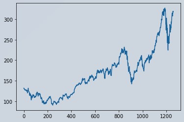
Figure 1 : Apple Stock Market Data Visualization
Scaling Data
Before we begin our model fitting, lets normalize this data. This will boost the performance. It is clear that the df1 is a vector. But the problem is MinMaxScaler works on numpy 2D arrays, not on vectors. So, we will convert df1 to 2D array using np.array(df1).reshape(-1,1)) and then apply the scaling.
    df1 = np.array(df1)
    df1 = df1.reshape(-1,1)

    scaler = MinMaxScaler(feature_range=(0,1))
    df1 = scaler.fit_transform(df1)
    print(df1)

[[0.17607447]
 [0.17495567]
 [0.16862282]
 ...
 [0.96635143]
 [0.9563033 ]
 [0.96491598]]
Splitting Data into Training and Testing Set
    df1.shape
(1258, 1)
In this analysis we will split the dataset into 65% training and 35% testing set. Lets split our data into training and testing sets as a standard process.
    # splitting dataset into train and test split
    training_size = int(len(df1)*0.65)
    test_size = len(df1)-training_size
    train_data,test_data  =df1[0:training_size,:], df1[training_size:len(df1),:1]
    train_data.shape
(817, 1)

    test_data.shape
(441, 1)

    training_size, test_size
(817, 441)

    train_data[:10]
array([[0.17607447],
       [0.17495567],
       [0.16862282],
       [0.1696994 ],
       [0.16727181],
       [0.16794731],
       [0.16473866],
       [0.16174111],
       [0.1581525 ],
       [0.15654817]])
Converting Array of Matrix into a Dataset Matrix
Now we will write a function that will prepare the dataset so that we can fit it easily in the Linear Regression model.
Windowing Dataset
For better performance of any time series (univariate), it is necessary to use the splitting window on the dataset. The concept is simple. We will convert the dataset into several overlapping series. You will have an idea by seeing the picture below.
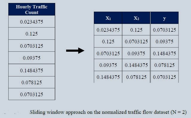
Figure 2 : Specimen Sliding Window Approach on Normalized Traffic Flow Data
Figure 2, shows the window size = 2. We will be using suitable window size for the best performance. You can try with any number you want. It is a hyper parameter that is needed to be tuned.
    def create_dataset(dataset, time_step=1):
        dataX, dataY = [], []
        for i in range(len(dataset)-time_step-1):
            a= dataset[i:(i+time_step), 0]
            dataX.append(a)
            dataY.append(dataset[i+ time_step, 0])
        return np.array(dataX), np.array(dataY)
Let's choose window size = 100 for now and apply the windowing on training and testing data's
    time_step = 100
    X_train, y_train = create_dataset(train_data, time_step)
    X_test, y_test = create_dataset(test_data, time_step)
    train_data.shape, test_data.shape
((817, 1), (441, 1))
    # A total of 817 + 441 = 1258
    # allocate series of 817  from index 1 to 817
    trainplot = np.arange(1,818)
    # allocate series of 818 to 1258
    testplot = np.arange(818,1259)
    # Ploting Train and Test Data
    plt.figure(figsize=(12,8))
    plt.plot(trainplot,scaler.inverse_transform(train_data)[:,0], 'green', label='Train data')
    plt.plot(testplot, scaler.inverse_transform(test_data)[:,0],'blue', label='Test data')
    plt.legend()
    plt.title('Train and Test Data')
    plt.show()
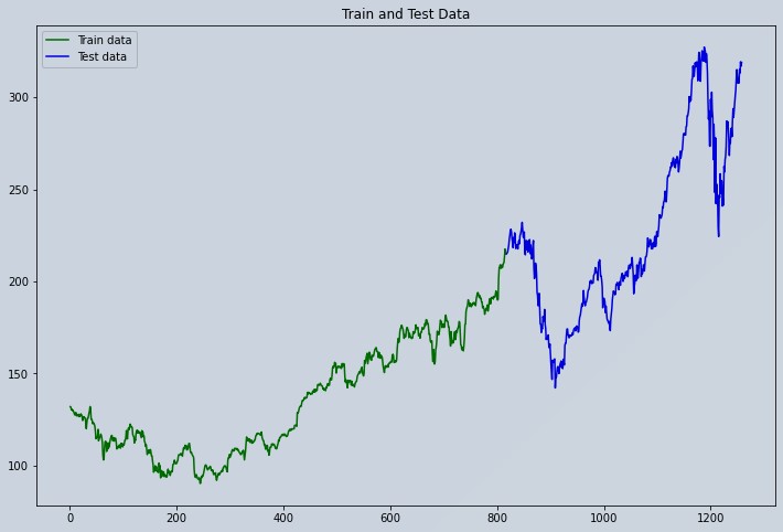
Figure 3 : Apple Stock Market Data Visualization Train and Test Series
Model Building (linear Regression)
Now it's time to build our model ::::: LinearRegression
    model = LinearRegression()
    model.fit(X_train, y_train)

LinearRegression()
Predictions and Model Evaluation
Predictions of Testing Set ::::: Now we visualize how our models perform within the test set
    predictions = model.predict(X_test)
    print("Predicted Value",predictions[:10][0])
    print("Expected Value",y_test[:10][0])

Predicted Value 0.26591241262096627
Expected Value 0.2727349489149709

    pred_df= pd.DataFrame(predictions)
    pred_df['TrueValues']=y_test

    new_pred_df=pred_df.rename(columns={0: 'Predictions'})
    new_pred_df.head()

Predictions  TrueValues
0     0.265912    0.272735
1     0.267869    0.276619
2     0.289373    0.280672
3     0.286837    0.265811
4     0.264365    0.268429
Plot Predicted vs Actual Prices of Test Series
    plt.figure(figsize=(12,8))
    sns.lineplot(data=new_pred_df)
    plt.title("Predictions Vs True Values on Testing Set")

Text(0.5, 1.0, 'Predictions Vs True Values on Testing Set')
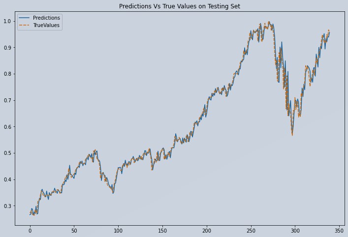
Figure 4: Plot of Predicted vs Actual Apple Stock Test Data
    print("model Accuracy on training data:",model.score(X_train, y_train))

model Accuracy on training data: 0.9970342320018716

    # Model accuracy on Testing data
    print("model Accuracy is on training data:",model.score(X_test, y_test))

model Accuracy on testing data: 0.9847722212152704

    # Lets Do the prediction and check performance metrics
    train_predict = model.predict(X_train)
    test_predict = model.predict(X_test)
    train_predict = train_predict.reshape(-1, 1)
    test_predict = test_predict.reshape(-1, 1)

    # Transform back to original form
    train_predict = scaler.inverse_transform(train_predict)
    test_predict = scaler.inverse_transform(test_predict)

    # Calculate RMSE performance metrics
    math.sqrt(mean_squared_error(y_train,train_predict))
142.1363100026703

    # Test Data RMSE
    math.sqrt(mean_squared_error(y_test,test_predict))
238.13157949250507
Conclusion
Our model performed good at predicting the Apple Stock price using a Linear Regression model. This entire code stack can be reused in any stock price prediction. This prediction is only short-term. We wont recommend to use this model for medium to long term forecast periods, as it depreciates in performance. Not because our Linear model is bad, but, because Stock markets are highly volatile. Read through this implementation of Stock price prediction using LSTM.
About the Author's:
Write A Public Review