Table of Content
Linear Regression
What is Linear Regression used for ?
Why is linear regression a Supervised Machine Learning Algorithm ?
What are the types of linear regression?
Simple Linear Regression
Multiple Linear Regression
How do you calculate parameters of simple linear regression?
Scatter plot
General trend of a linear regression line
Case study (University admission prediction)
Step1: Plotting a scatter chart
Step 2: Calculating the residuals
Step 3: Calculating the slope
Step 4: Calculating the estimated value of y (chance of admit) using test dataset
What is R Square and how do you interpret R Squared in regression analysis?
Implementing Linear Regression from scratch in Python
Linear Regression
It is a type of predictive modelling technique based on statistics, created to predict the value of a specific entity based on historical data. It is a supervised machine learning algorithm. It is used to predict the value of a continuous variable also known as target variable or response variable based on one or more than one predictor (also known as features or independent variables).
What is linear regression used for?
Linear regression can be used in different sectors viz. in real estate sector for the valuation of a property, in the retail sector for predicting monthly sales and the price of goods, for estimating the salary of an employee, in the educational sector for predicting the %marks of a student in the final exam based on his previous performance, etc. Financial forecasting is a classic application of regression that uses related information to predict the future value of entities like revenues, expenses, exchange rates, and capital costs.
Why is linear regression a supervised machine learning algorithm ?
Linear regression is a supervised machine learning technique in which the system is trained with the target variable for identifying the trend before it can predict the outcome with unknown feature variable.
For example, consider the diagram below, in which a training model is constructed consisting of a single feature variable which is GRE score, and a target variable which is the % chance of getting admission into the University.
Once the machine is trained with the specified model, the system can predict the target variable (% change of getting admission) based on the test dataset containing unlabelled GRE score as specified in the diagram below.
Figure 1 : Linear Model predicting using Features and Target variable on Test Data
What are the types of linear regression?
There are primarily two types of linear regression, simple linear regression and multiple linear regression.
Simple Linear Regression
In simple linear regression a single feature variable or predictor determines the value of target variable or the outcome.
The equation is:
Multiple Linear Regression
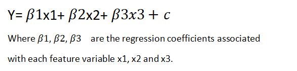
In Multiple linear regression, multiple feature variables are involved in determining the outcome or the value of target variable.
The equation is as follows: -
How do you calculate parameters of simple linear regression?
Linear regression models the linear relationship between two variables using a simple regression line which is a straight line. The two variables here are the independent variable, which is the cause and the dependant variable also known as the output, target or the response variable which depicts the effect.
For example, let us consider two variables which are linearly related. We need to find a linear function that predicts the response value(y) with the help of its feature variable or independent variable(x).
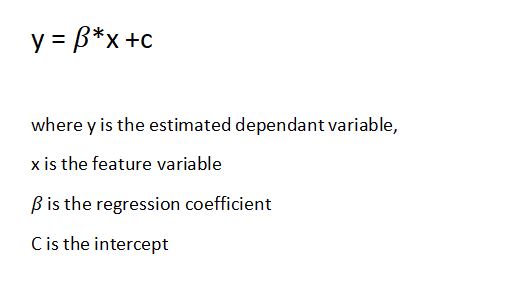
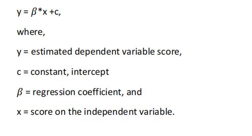
The simple linear regression equation with one dependent or feature variable and one independent or response variable is defined by the formula
We have a sample data set in which value of response y against every feature x is tabulated as in Figure 2:
x as feature vector
y as response vector
Figure 2: Table of sample data
Scatter plot
A scatter chart helps to visualize the response against every feature and we are trying to draw a line draw covering most of the data points. We can also call this as a regression line.
Figure 3: Scatter Plot and Straight Linear Line Passing through data
General trend of a linear regression line
A regression line is a straight line depicting the linear relationship between the two variables and is represented by a regression coefficient( ß) which is also the slope of the line, and the intercept which is also labelled as constant and is the expected mean value of y when all x=0.
There can be 3 different scenarios:
1. When there is no change in the value of y with respect to change in the value of x, ß is 0.
2. With increase in value of x, the value of y increases (x is directly proportional to y), ß is +ve.
3. With increase in value of x, y decreases (x is inversely proportional to y), ß is -ve.
Figure 4 : Trend of Linear Regression Line
Case study (University admission prediction)
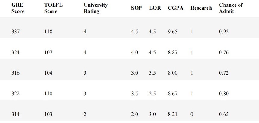
The University Admission Prediction dataset contains several parameters which are considered important during the application for Masters Programs. The data is available on kaggle. We have kept a copy of the University Admission Prediction dataset here.
For Simple linear regression let us consider the “GRE Score” (out of 340) as the feature which influences the “chance of admit” which ranges from 0 to 1.
Step1: Plotting a scatter chart
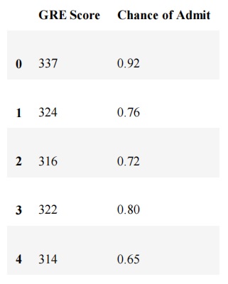
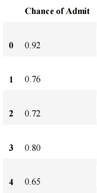
Plot a scatter chart to analyse the relationship between the variables. Linear regression is possible only if a linear relationship between the two variables exists. In scatter chart the points should fall along a line and not be like a blob. We have taken only the first 5 records here for analysis.
GRE score
Chance of admit
337
0.92
324
0.76
316
0.72
322
0.8
314
0.65
Figure 5 : Snapshot of top 5 Records in University Admission Dataset
Figure 6 : Scatterplot of top 5 Records in University Admission Dataset along with linear line
Step 2: Calculating the Residuals
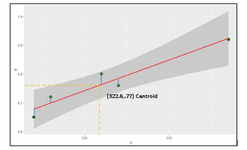
Now that we know there is a linear relationship between x and y, the system looks for a best fit regression line which minimise the residuals. Residuals are deviations of the actual data points from the regression line. The best fit line will have minimum residuals.
The regression line is sometimes called the "line of best fit" or the "best fit line". Since it "best fits" the data, the line passes through the mean of x and mean of y called the centroid.
GRE score ( X )
Chance of Admit ( Y )
Deviation GRE score
(Xi-mean(Xi))
Deviation Chance of Admit
(Yi-mean(Yi))
337
0.92
14.4
0.15
324
0.76
1.4
-0.01
316
0.72
-6.6
-0.05
322
0.8
-0.6
0.03
314
0.65
-8.6
-0.12
Mean (Xi)
Mean (Yi)
322.6
0.77
Figure 7 : Manual Computations for the Linear Regression Line
Figure 8 : Graph showing Computation of residuals in Linear Regression
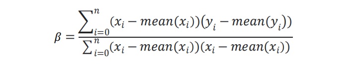
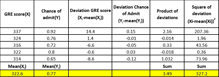
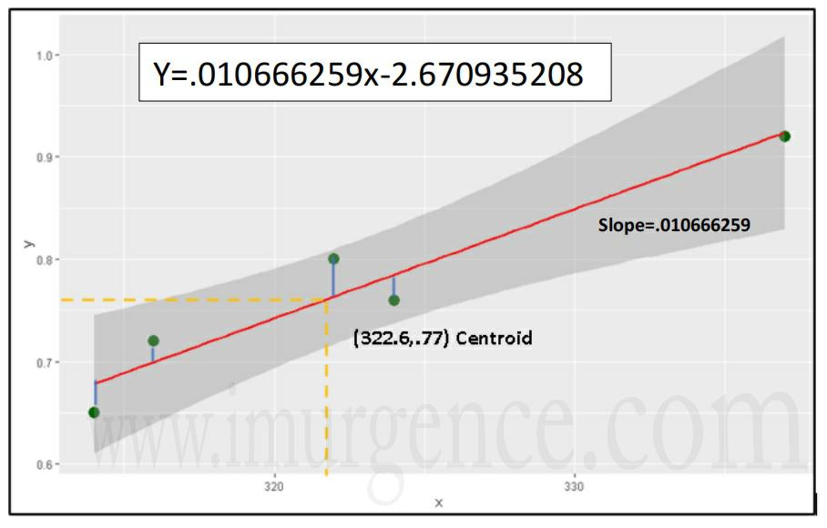
Step 3: Calculating the Slope
Calculate the slope of the line using the following equation: -
Figure 9 : Table of University Admission Dataset beta compuation
ß = 3.49/327.2
= 0.010666259
As per the equation
y = ß*x +c
By substituting mean(x) and mean(y) in the equation, we get the value of the intercept (c)
c = 0.77 - 0.010666259 * 322.6
= - 2.670935208
Final equation:
Y = 0.010666259x - 2.670935208
Figure 10 : Regression line in University Admission Dataset along with the slope represenation
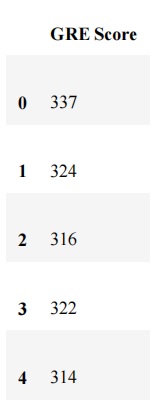
Step 4 : Calculating the estimated value of y (chance of admit) using test dataset
GRE Score
Chance of
admit
320
?
325
?
Y1 = 0.010666259 * 320 - 2.670935208
Y1 = 0.742267672
Y2 = 0.010666259 * 325 - 2.670935208
Y2 = 0.795598967
What is R Square and how do you interpret R Squared in regression analysis?
R Square is also known as coefficient of determination and is a measure of the goodness of fit of the regression line to existing data points. The value of R Square ranges from 0 to 1.
If R Square is 1 then all the data points fall perfectly on the Regression line.
If R Square is 0, the regression line is horizontal. The predictor p does not account for any variation in the target variable y.
If R Square is between 0 and 1, the predictor p accounts for R2 *100 percent variation in the target variable y.
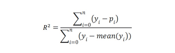
R square is represented by the following formula
Where,
yi is the target or response variable in the test dataset and pi is the predicted response variable. R - square is calculated in the training dataset to understand the accuracy of the model.
Implementing Linear Regression from scratch in Python
import pandas as pd
import the dataset
df_admit=pd.read_csv("c:/csv/admission_predict.csv")
Extracting the first 5 records
df1=df_admit.head(5)
df1
Selecting the GRE Score and the Chance of admit column
df1=df1.iloc[:,[1,7]]
df1
setting GRE score as X vector
df1_x=df1.iloc[:,[0]]
df1_x
converting object to numeric column
x=df1_x.iloc[:,0]
x=pd.to_numeric(x)
setting Chance of admit as Y vector
df1_y=df1.iloc[:,[1]]
df1_y
converting object to numeric column
y=df1_y.iloc[:,0]
import numpy as np
calculating the mean of x and y vectors
df1_x_mean=np.mean(df1_x)
df1_x_mean
df1_y_mean=np.mean(df1_y)
df1_y_mean
calculating the deviation in x
deviation_x=[]
for i in x:
deviation_x.append(i-df1_x_mean)
deviation_x
calculating the deviation in y
deviation_y=[]
for i in y:
deviation_y.append(i-df1_y_mean)
deviation_y
calculating the product of deviations
product_deviation=np.array(deviation_x)*np.array(deviation_y)

product_deviation

Sum_product_deviation=np.sum(product_deviation)
Sum_product_deviation
calculating the square of deviation of x and y
Sq_x_deviation=np.array(deviation_x)**2

Sq_x_deviation

Sum_Sq_x_deviation=np.sum(Sq_x_deviation)
Sum_Sq_x_deviation
calculating the regression coefficient, the slope of regression line
Regression_coefficient=Sum_product_deviation/Sum_Sq_x_deviation

Regression_coefficient
calculating the intercept
intercept=np.float(df1_y_mean)-(Regression_coefficient*np.float(df1_x_mean))

intercept
calculating the predicted value of y from test data
predicted_y1=Regression_coefficient*test_data[0]+intercept

predicted_y1


predicted_y2=Regression_coefficient*test_data[1]+intercept
predicted_y2
Implementing linear regression with SKLearn library
from sklearn.linear_model import LinearRegression
model1=LinearRegression()
#training the model with X as feature and Y as target
model1=model1.fit(df1_x,df1_y)
printing the regression coefficient or the slope of the regression line
print(model1.coef_)
printing the intercept
print(model1.intercept_)
creating the test dataset
x_test=pd.DataFrame({"GRE Score":[320,325]})
Predicting the value of Y (Chance of admit)
p=model1.predict(x_test)
p
Calculating R2_score
from sklearn.metrics import r2_score
The target variable of the test dataset is unknown so we need to use the training dataset
p_tr=model1.predict(df1_x)
r2_score(df1_y,p_tr)
We have done this implemenation on the top 5 records of the dataset. As a next step you should implement the same on the complete data set.
About the Author:
Indrani Sen
Indrani Sen is an Academician, Freelance Machine learning and coding instructor, and Ph.D. research scholar in the University of Mumbai. She has more than 15 years of experience in Teaching Computer Science and IT in various leading colleges and the University of Mumbai. As a machine learning trainer, she has worked with various clients like Tata Consultancy Services, Great Lakes Institute of Management, Regenesys Business school, etc. to name a few.
Table of Content
- Linear Regression
- What is Linear Regression used for ?
-
-
-
-
-
-
-
-
-
-
-
-
-
-
It is a type of predictive modelling technique based on statistics, created to predict the value of a specific entity based on historical data. It is a supervised machine learning algorithm. It is used to predict the value of a continuous variable also known as target variable or response variable based on one or more than one predictor (also known as features or independent variables).
Linear regression can be used in different sectors viz. in real estate sector for the valuation of a property, in the retail sector for predicting monthly sales and the price of goods, for estimating the salary of an employee, in the educational sector for predicting the %marks of a student in the final exam based on his previous performance, etc. Financial forecasting is a classic application of regression that uses related information to predict the future value of entities like revenues, expenses, exchange rates, and capital costs.
Linear regression is a supervised machine learning technique in which the system is trained with the target variable for identifying the trend before it can predict the outcome with unknown feature variable.
For example, consider the diagram below, in which a training model is constructed consisting of a single feature variable which is GRE score, and a target variable which is the % chance of getting admission into the University.
Once the machine is trained with the specified model, the system can predict the target variable (% change of getting admission) based on the test dataset containing unlabelled GRE score as specified in the diagram below.
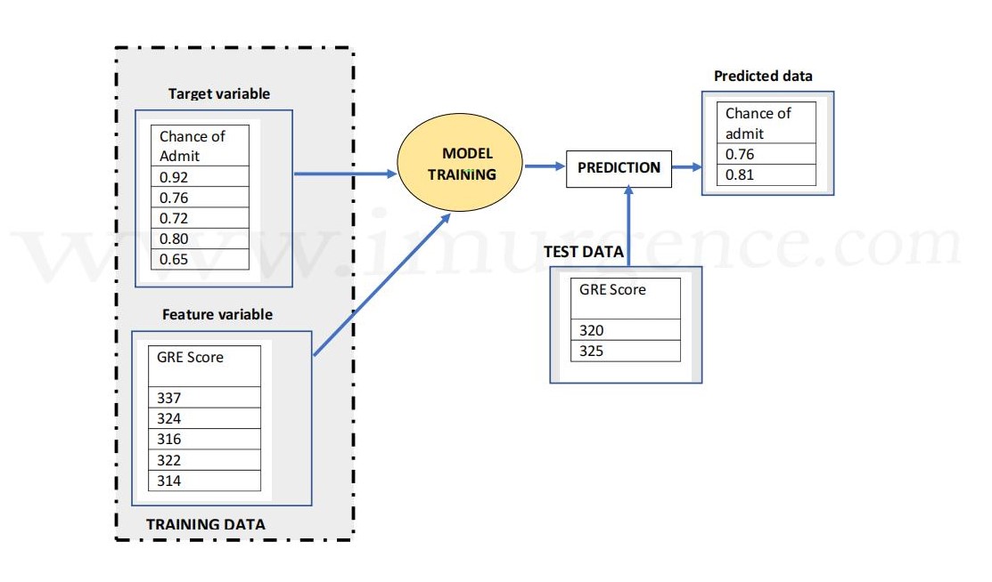
Figure 1 : Linear Model predicting using Features and Target variable on Test Data
There are primarily two types of linear regression, simple linear regression and multiple linear regression.
In simple linear regression a single feature variable or predictor determines the value of target variable or the outcome.
The equation is:
In Multiple linear regression, multiple feature variables are involved in determining the outcome or the value of target variable.
The equation is as follows: -
Linear regression models the linear relationship between two variables using a simple regression line which is a straight line. The two variables here are the independent variable, which is the cause and the dependant variable also known as the output, target or the response variable which depicts the effect.
For example, let us consider two variables which are linearly related. We need to find a linear function that predicts the response value(y) with the help of its feature variable or independent variable(x).
The simple linear regression equation with one dependent or feature variable and one independent or response variable is defined by the formula
We have a sample data set in which value of response y against every feature x is tabulated as in Figure 2:
x as feature vector
y as response vector
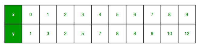 Figure 2: Table of sample data
A scatter chart helps to visualize the response against every feature and we are trying to draw a line draw covering most of the data points. We can also call this as a regression line.
 Figure 3: Scatter Plot and Straight Linear Line Passing through data
A regression line is a straight line depicting the linear relationship between the two variables and is represented by a regression coefficient( ß) which is also the slope of the line, and the intercept which is also labelled as constant and is the expected mean value of y when all x=0.
There can be 3 different scenarios:
1. When there is no change in the value of y with respect to change in the value of x, ß is 0.
2. With increase in value of x, the value of y increases (x is directly proportional to y), ß is +ve.
3. With increase in value of x, y decreases (x is inversely proportional to y), ß is -ve.
 Figure 4 : Trend of Linear Regression Line
The University Admission Prediction dataset contains several parameters which are considered important during the application for Masters Programs. The data is available on kaggle. We have kept a copy of the University Admission Prediction dataset here.
For Simple linear regression let us consider the “GRE Score” (out of 340) as the feature which influences the “chance of admit” which ranges from 0 to 1.
Plot a scatter chart to analyse the relationship between the variables. Linear regression is possible only if a linear relationship between the two variables exists. In scatter chart the points should fall along a line and not be like a blob. We have taken only the first 5 records here for analysis.
| GRE score |
Chance of admit |
|
337
|
0.92
|
|
324
|
0.76
|
|
316
|
0.72
|
|
322
|
0.8
|
|
314
|
0.65
|
Figure 5 : Snapshot of top 5 Records in University Admission Dataset
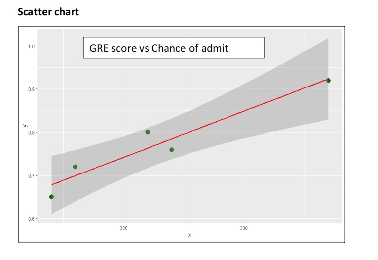 Figure 6 : Scatterplot of top 5 Records in University Admission Dataset along with linear line
Now that we know there is a linear relationship between x and y, the system looks for a best fit regression line which minimise the residuals. Residuals are deviations of the actual data points from the regression line. The best fit line will have minimum residuals.
The regression line is sometimes called the "line of best fit" or the "best fit line". Since it "best fits" the data, the line passes through the mean of x and mean of y called the centroid.
| GRE score ( X ) |
Chance of Admit ( Y ) |
Deviation GRE score
(Xi-mean(Xi))
|
Deviation Chance of Admit
(Yi-mean(Yi))
|
|
337
|
0.92
|
14.4
|
0.15
|
|
324
|
0.76
|
1.4
|
-0.01
|
|
316
|
0.72
|
-6.6
|
-0.05
|
|
322
|
0.8
|
-0.6
|
0.03
|
|
314
|
0.65
|
-8.6
|
-0.12
|
|
Mean (Xi)
|
Mean (Yi)
|
|
|
|
322.6
|
0.77
|
|
|
Figure 7 : Manual Computations for the Linear Regression Line
Figure 8 : Graph showing Computation of residuals in Linear Regression
Calculate the slope of the line using the following equation: -
Figure 9 : Table of University Admission Dataset beta compuation
ß = 3.49/327.2
= 0.010666259
As per the equation
y = ß*x +c
By substituting mean(x) and mean(y) in the equation, we get the value of the intercept (c)
c = 0.77 - 0.010666259 * 322.6
= - 2.670935208
Final equation:
Y = 0.010666259x - 2.670935208
Figure 10 : Regression line in University Admission Dataset along with the slope represenation
|
GRE Score
|
Chance of
admit
|
|
320
|
?
|
|
325
|
?
|
Y1 = 0.010666259 * 320 - 2.670935208
Y1 = 0.742267672
Y2 = 0.010666259 * 325 - 2.670935208
Y2 = 0.795598967
R Square is also known as coefficient of determination and is a measure of the goodness of fit of the regression line to existing data points. The value of R Square ranges from 0 to 1.
If R Square is 1 then all the data points fall perfectly on the Regression line.
If R Square is 0, the regression line is horizontal. The predictor p does not account for any variation in the target variable y.
If R Square is between 0 and 1, the predictor p accounts for R2 *100 percent variation in the target variable y.
R square is represented by the following formula
Where,
yi is the target or response variable in the test dataset and pi is the predicted response variable. R - square is calculated in the training dataset to understand the accuracy of the model.
import pandas as pd
import the dataset
df_admit=pd.read_csv("c:/csv/admission_predict.csv")
Extracting the first 5 records
df1=df_admit.head(5)
df1
Selecting the GRE Score and the Chance of admit column
setting GRE score as X vector
df1_x=df1.iloc[:,[0]]
df1_x
converting object to numeric column
setting Chance of admit as Y vector
converting object to numeric column
y=df1_y.iloc[:,0]
import numpy as np
calculating the mean of x and y vectors
df1_x_mean=np.mean(df1_x)
df1_x_mean
df1_y_mean=np.mean(df1_y)
calculating the deviation in x
deviation_x=[]
for i in x:
deviation_x.append(i-df1_x_mean)
calculating the deviation in y
deviation_y=[]
for i in y:
deviation_y.append(i-df1_y_mean)
deviation_y
calculating the product of deviations
product_deviation=np.array(deviation_x)*np.array(deviation_y)
product_deviation
Sum_product_deviation=np.sum(product_deviation)
Sum_product_deviation
calculating the square of deviation of x and y
Sq_x_deviation=np.array(deviation_x)**2
Sq_x_deviation
Sum_Sq_x_deviation=np.sum(Sq_x_deviation)
Sum_Sq_x_deviation
calculating the regression coefficient, the slope of regression line
Regression_coefficient=Sum_product_deviation/Sum_Sq_x_deviation
calculating the intercept
intercept=np.float(df1_y_mean)-(Regression_coefficient*np.float(df1_x_mean))
calculating the predicted value of y from test data
predicted_y1=Regression_coefficient*test_data[0]+intercept
predicted_y1
predicted_y2=Regression_coefficient*test_data[1]+intercept
predicted_y2
Implementing linear regression with SKLearn library
from sklearn.linear_model import LinearRegression
model1=LinearRegression()
#training the model with X as feature and Y as target
model1=model1.fit(df1_x,df1_y)
printing the regression coefficient or the slope of the regression line
printing the intercept
creating the test dataset
x_test=pd.DataFrame({"GRE Score":[320,325]})
Predicting the value of Y (Chance of admit)
Calculating R2_score
from sklearn.metrics import r2_score
The target variable of the test dataset is unknown so we need to use the training dataset
p_tr=model1.predict(df1_x)
We have done this implemenation on the top 5 records of the dataset. As a next step you should implement the same on the complete data set.
About the Author:

Write A Public Review