How To Use Convolution Neural Network For Image Classification On Mnist Fashion Dataset.

Table of Content

Introduction
Importing Libraries
Data Visualization
Data Pre-Processing
Building Model
Model Summary
Training Model
Evaluating Model
Predictions Through Model
Predictions Using Real Time Data
Confusion Matrix
Heatmap
Conclusion and Summary

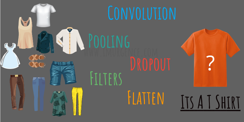
Introduction

Convolution Neural Network (CNN) is a deep learning algorithm which takes image as an input then applies feature extraction on it through different hidden layers of neural network and be able to differentiate it from other images. Here the task of labeling the images is done by hidden layers present in our network. The architecture of CNN is similar to that of neurons present in a human brain. We intend to use the CNN implementation to create a automated tagging workflow which identifies the fashion apparel in the inventory of an online or offline retail store. This would reduce the time taken for human classification of inventory.

Various Layers of CNN are –

Input
Feature Extraction
1. Convolution + RELU(Rectified Linear Unit)
2. Pooling
3. Dropout
Classification
1. Flatten
2. Fully Connected
3. Dropout
4. Softmax
Output

Importing Libraries

    # Importing Libraries and Dataset
    import pandas as pd
    import numpy as np
    import matplotlib.pyplot as plt
    import seaborn as sns
    import keras
    import cv2
    from keras.layers import Dropout
    from keras.datasets import fashion_mnist
    from keras.utils import to_categorical
    from keras.models import Sequential
    from keras.layers import Conv2D, MaxPooling2D, Flatten, Dense
    from keras.optimizers import Adam
    from sklearn.metrics import confusion_matrix, classification_report
    
    # Load the fashion-mnist data and Split into train test 
    (X_train, Y_train), (X_test, Y_test) = fashion_mnist.load_data()

Downloading data from https://storage.googleapis.com/tensorflow/tf-keras-datasets/train-labels-idx1-ubyte.gz
32768/29515 [=================================] - 0s 2us/step
Downloading data from https://storage.googleapis.com/tensorflow/tf-keras-datasets/train-images-idx3-ubyte.gz
26427392/26421880 [==============================] - 14s 1us/step
Downloading data from https://storage.googleapis.com/tensorflow/tf-keras-datasets/t10k-labels-idx1-ubyte.gz
8192/5148 [===============================================] - 0s 0us/step
Downloading data from https://storage.googleapis.com/tensorflow/tf-keras-datasets/t10k-images-idx3-ubyte.gz
4423680/4422102 [==============================] - 3s 1us/step

    X_train.shape
(60000, 28, 28)

    X_test.shape
(10000, 28, 28)

    Y_train.shape
(60000,)

    Y_test.shape
(10000,)

Data Visualization

There are 10 different classes of images, as following:

Label 0 : T-shirt/top

Label 1: Trouser

Label 2: Pullover

Label 3: Dress

Label 4: Coat

Label 5: Sandal

Label 6: Shirt

Label 7: Sneaker

Label 8: Bag

Label 9: Ankle boot

    plt.imshow(np.reshape(X_train[1], (28,28)), cmap = 'gray')
    plt.title("Label: %i" %Y_train[1])
    plt.show()

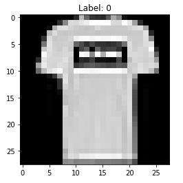
Figure 1 : Image Sample 1 from MNIST fashion dataset

    plt.imshow(np.reshape(X_train[650], (28,28)), cmap = 'gray')
    plt.title("Label: %i" %Y_train[650])
    plt.show()

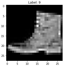
Figure 2 : Image Sample 2 from MNIST fashion dataset

    Y_train[0:10]
array([9, 0, 0, 3, 0, 2, 7, 2, 5, 5], dtype=uint8)

Data Pre-Processing

    # Define Labels 
    fashion_labels = ['T-shirt/top',
                      'Trouser',
                      'Pullover',
                      'Dress',
                      'Coat',
                      'Sandal',
                      'Shirt',
                      'Sneaker',
                      'Bag',
                      'Ankle boot']
    
    # Image pixel Normalization
    X_train = X_train.astype('float32')/255
    X_test = X_test.astype('float32')/255
    
    X_train[0]
    
    image_height = 28
    image_width = 28
    
    # Grayscale image with num_channels (Rank = 1)
    num_channels = 1
    
    # Reshaping of Image = (60000, 28, 28, 1)
    train_digits = np.reshape(X_train, newshape=(60000, image_height, image_width, num_channels))
    test_digits = np.reshape(X_test, newshape=(10000, image_height, image_width, num_channels))
    
    # 0 - 9 num_classes = 10
    # 7 - [0, 0, 0, 0, 0, 0, 0, 1, 0, 0]
    # 5 - [0, 0, 0, 0, 0, 1, 0, 0, 0, 0]
    
    num_classes = 10
    train_labels_class = to_categorical(Y_train, num_classes)
    test_labels_class = to_categorical(Y_test, num_classes)
    train_labels_class

array([[0., 0., 0., ..., 0., 0., 1.],
       [1., 0., 0., ..., 0., 0., 0.],
       [1., 0., 0., ..., 0., 0., 0.],
       ...,
       [0., 0., 0., ..., 0., 0., 0.],
       [1., 0., 0., ..., 0., 0., 0.],
       [0., 0., 0., ..., 0., 0., 0.]], dtype=float32)

Building Model

    def build_model():
    model = Sequential()
    
    # Layer - I (Padding = 'same' --> zero padding)
    model.add(Conv2D(filters = 32, kernel_size=(3,3), strides=(1,1), padding = 'same', activation='relu', 
                       input_shape = (image_height, image_width, num_channels)))
    model.add(MaxPooling2D(pool_size=(2,2)))
    model.add(Dropout(0.25))
    
    model.add(Conv2D(filters = 64, kernel_size=(3,3), strides=(1,1), padding = 'same', activation='relu'))
    model.add(MaxPooling2D(pool_size=(2,2)))
    model.add(Dropout(0.25))
    
    model.add(Conv2D(filters = 128, kernel_size=(3,3), strides=(1,1), padding = 'same', activation='relu'))
    model.add(MaxPooling2D(pool_size=(2,2)))
    model.add(Dropout(0.25))
    
    # Flatten Matrix
    model.add(Flatten())
    
    # Fully Connected Layer
    model.add(Dense(units=128, activation='relu'))
    model.add(Dropout(0.30))
    
    # Output Layer
    model.add(Dense(units=10, activation='softmax'))
    
    # Model Compile
    optimizers = Adam(learning_rate = 0.001)
    
    # categorical_crossentropy - used for multiclass classification
    model.compile(loss = 'categorical_crossentropy', optimizer = optimizers, metrics = ['accuracy'])
    return model
    
    model = build_model()

Model Summary

    model.summary()

Model: "sequential"                                              
_________________________________________________________________
Layer (type)                 Output Shape              Param #   
=================================================================
conv2d (Conv2D)              (None, 28, 28, 32)        320       
_________________________________________________________________
max_pooling2d (MaxPooling2D) (None, 14, 14, 32)        0         
_________________________________________________________________
dropout (Dropout)            (None, 14, 14, 32)        0         
_________________________________________________________________
conv2d_1 (Conv2D)            (None, 14, 14, 64)        18496     
_________________________________________________________________
max_pooling2d_1 (MaxPooling2 (None, 7, 7, 64)          0         
_________________________________________________________________
dropout_1 (Dropout)          (None, 7, 7, 64)          0         
_________________________________________________________________
conv2d_2 (Conv2D)            (None, 7, 7, 128)         73856     
_________________________________________________________________
max_pooling2d_2 (MaxPooling2 (None, 3, 3, 128)         0         
_________________________________________________________________
dropout_2 (Dropout)          (None, 3, 3, 128)         0         
_________________________________________________________________
flatten (Flatten)            (None, 1152)              0         
_________________________________________________________________
dense (Dense)                (None, 128)               147584    
_________________________________________________________________
dropout_3 (Dropout)          (None, 128)               0         
_________________________________________________________________
dense_1 (Dense)              (None, 10)                1290      
=================================================================
Total params: 241,546                                            
Trainable params: 241,546                                        
Non-trainable params: 0                                          
_________________________________________________________________

Training Model

    result = model.fit(train_digits, train_labels_class, epochs=50, batch_size=64, validation_split=0.1)

Epoch 1/50
844/844 [==============================] - 70s 80ms/step - loss: 0.9277 - accuracy: 0.6530 - val_loss: 0.3862 - val_accuracy: 0.8540
Epoch 2/50
844/844 [==============================] - 77s 92ms/step - loss: 0.4095 - accuracy: 0.8517 - val_loss: 0.3166 - val_accuracy: 0.8808
Epoch 3/50
844/844 [==============================] - 81s 96ms/step - loss: 0.3535 - accuracy: 0.8710 - val_loss: 0.2824 - val_accuracy: 0.8957
Epoch 4/50
844/844 [==============================] - 81s 96ms/step - loss: 0.3218 - accuracy: 0.8808 - val_loss: 0.2593 - val_accuracy: 0.9037
Epoch 5/50
844/844 [==============================] - 79s 93ms/step - loss: 0.3020 - accuracy: 0.8852 - val_loss: 0.2501 - val_accuracy: 0.9062
...
...
...
...
...
Epoch 45/50
844/844 [==============================] - 108s 128ms/step - loss: 0.1585 - accuracy: 0.9389 - val_loss: 0.1922 - val_accuracy: 0.9283
Epoch 46/50
844/844 [==============================] - 99s 117ms/step - loss: 0.1595 - accuracy: 0.9394 - val_loss: 0.1901 - val_accuracy: 0.9305
Epoch 47/50
844/844 [==============================] - 80s 95ms/step - loss: 0.1565 - accuracy: 0.9402 - val_loss: 0.1953 - val_accuracy: 0.9295
Epoch 48/50
844/844 [==============================] - 81s 95ms/step - loss: 0.1540 - accuracy: 0.9411 - val_loss: 0.1937 - val_accuracy: 0.9288
Epoch 49/50
844/844 [==============================] - 111s 132ms/step - loss: 0.1587 - accuracy: 0.9392 - val_loss: 0.2026 - val_accuracy: 0.9268
Epoch 50/50
844/844 [==============================] - 90s 107ms/step - loss: 0.1568 - accuracy: 0.9406 - val_loss: 0.1945 - val_accuracy: 0.9285

Model Evaluation

    model.evaluate(test_digits, test_labels_class)

313/313 [==============================] - 5s 15ms/step - loss: 0.2267 - accuracy: 0.9284
Out[11]: [0.22667253017425537, 0.9283999800682068]

    pd.DataFrame(result.history)

        loss  accuracy  val_loss  val_accuracy
0   0.270684  0.900074  0.235163      0.910500
1   0.262369  0.903852  0.235229      0.910667
2   0.254143  0.905611  0.225067      0.916833
3   0.244829  0.908963  0.227146      0.916833
4   0.237125  0.911722  0.220977      0.918167
5   0.231625  0.913889  0.219834      0.914667



45  0.159503  0.939389  0.190102      0.930500
46  0.156466  0.940204  0.195315      0.929500
47  0.153997  0.941148  0.193682      0.928833
48  0.158681  0.939167  0.202637      0.926833
49  0.156842  0.940630  0.194501      0.928500

    pd.DataFrame(result.history)[['accuracy', 'val_accuracy']].plot()

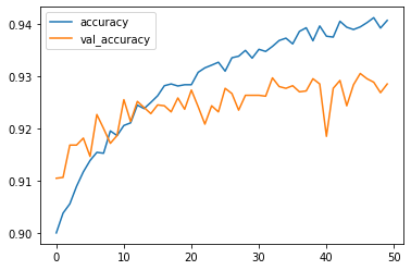
Accuracy Chart for model evaluation of CNN on MNIST fashion data

Figure 3 : Accuracy Chart for model evaluation of CNN on MNIST fashion data

    pd.DataFrame(result.history)[['loss', 'val_loss']].plot()

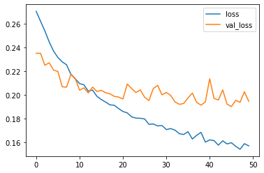
Loss Chart for model evaluation of CNN on MNIST fashion data

Figure 4 : Loss Chart for model evaluation of CNN on MNIST fashion data

Predictions Through the Model

    # Converts Categorical o/p into integar o/p
    yhat = np.argmax(predictions, axis = 1)
    yhat = np.argmax(model.predict(np.reshape(test_digits[5], (1, 28, 28, 1))))

    plt.imshow(np.reshape(test_digits[5], (28,28)), cmap = 'gray')
    plt.title("Label: %i Prediction: %i" %(Y_train[6], yhat))
    plt.show()

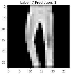
Predicted Image sample for CNN on MNIST fashion dataset

Figure 5 : Predicted Image sample for CNN on MNIST fashion dataset

Predictions Using Real Time Data

    # 0 - Gray Scale
    # sample data to ingest

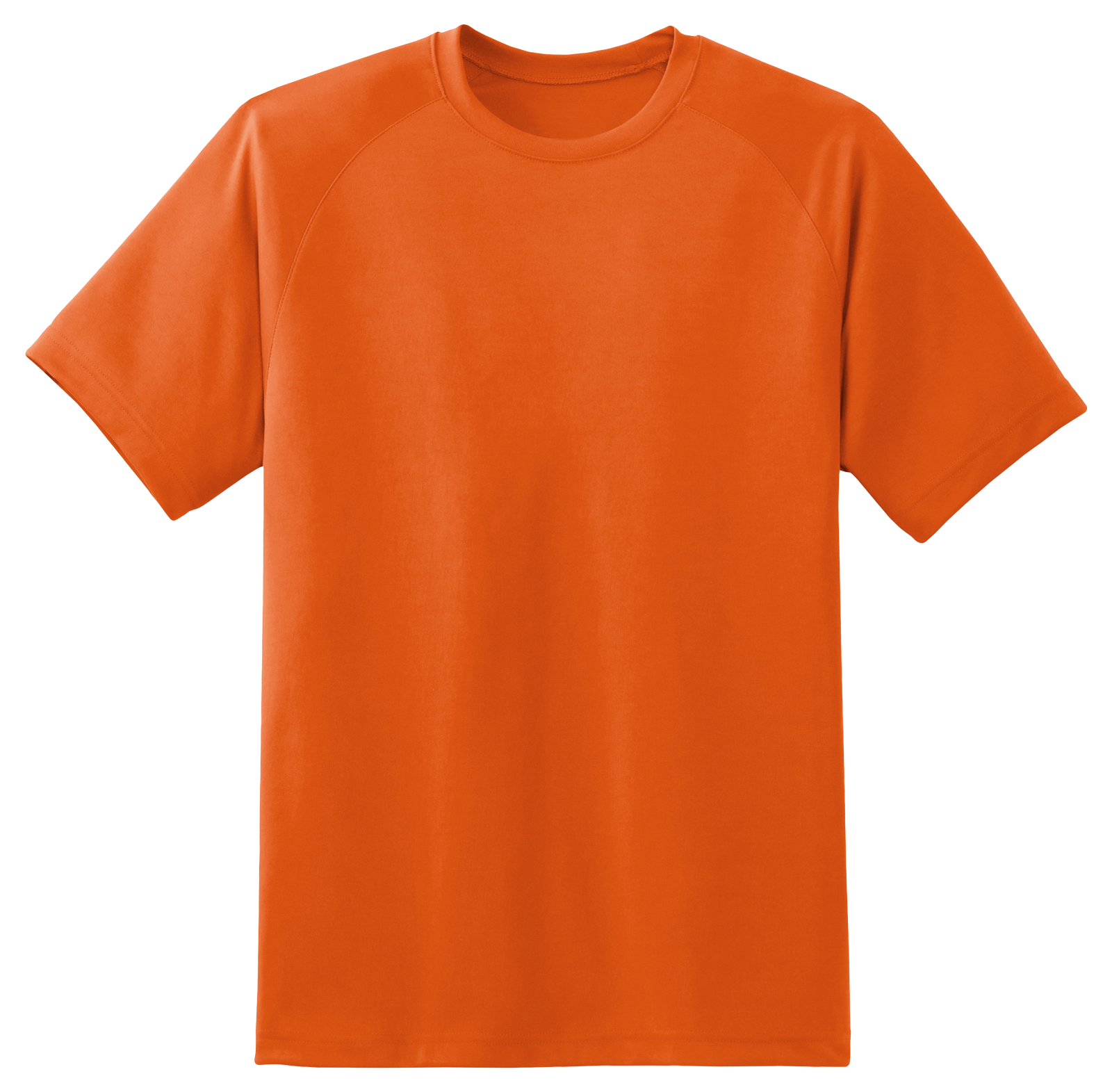
our data for testing CNN built on MNIST fashion dataset

Figure 6 : Our data for testing CNN built on MNIST fashion dataset

    img = cv2.imread('test-tshirt.jpg', 0)
    img.shape
(1571, 1600)

    test_digits.shape
(10000, 28, 28, 1)
         
    img_data = cv2.resize(img, (28, 28))
    plt.imshow(img_data, cmap = 'gray')
 
   
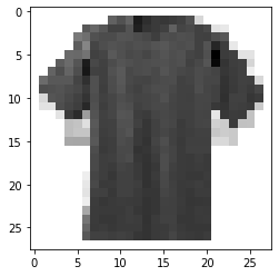Figure 7 : Ingest our data for testing CNN built on MNIST fashion dataset

    # Bitwise operation not for image samples 
    img_data = cv2.bitwise_not(img_data)
    img_new = np.reshape(img_data, (1, image_height, image_width, num_channels))
    model.predict(img_new)
    
array([[1.0000000e+00, 0.0000000e+00, 5.3774135e-33, 0.0000000e+00,
        0.0000000e+00, 0.0000000e+00, 0.0000000e+00, 0.0000000e+00,
        0.0000000e+00, 0.0000000e+00]], dtype=float32)             

    plt.imshow(img_data, cmap = 'gray')
    plt.title("Predicted O/P :%i" %np.argmax(model.predict(img_new)))

Text(0.5, 1.0, 'Predicted O/P :0')

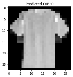
Figure 8 : Predicted Class of Ingested Image for CNN on MNIST Fashion dataset

Confusion Matrix

    predictions = model.predict(test_digits)
    yhat = np.argmax(predictions, axis = 1)
    confusion_matrix(Y_test, yhat)

array([[853,   0,  15,  11,   4,   1, 110,   0,   6,   0],
       [  0, 985,   0,   9,   2,   0,   3,   0,   1,   0],
       [ 18,   1, 872,   6,  56,   0,  46,   0,   1,   0],
       [  7,   4,   8, 940,  20,   0,  21,   0,   0,   0],
       [  0,   0,  21,  20, 907,   0,  52,   0,   0,   0],
       [  0,   0,   0,   0,   0, 987,   0,   9,   0,   4],
       [ 68,   0,  36,  27,  66,   0, 800,   0,   3,   0],
       [  0,   0,   0,   0,   0,   7,   0, 980,   0,  13],
       [  1,   1,   1,   2,   1,   2,   2,   0, 990,   0],
       [  0,   0,   0,   0,   0,   4,   1,  25,   0, 970]], dtype=int64)

Heatmap

    plt.figure(figsize = (10, 10))
    sns.heatmap(confusion_matrix(Y_test, yhat), annot = True, fmt = '0.0f')

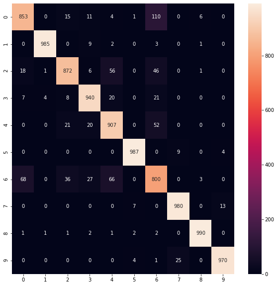
Cross Tabulation of CNN model on MNIST Fashion data

Figure 8 : Cross Tabulation of CNN model on MNIST Fashion data

Conclusion and Summary

In this tutorial we discussed how to predict apparels using Deep Learning Convolution Neural Network (CNN) in Python. Also, we learned how to build model, add different layers, train model and test model using MNIST Fashion Dataset. We also made some predictions by importing a real time image of a T-Shirt and out model predicted correct. An application like this can help in real time tagging for inventory management. Confusion matrix and Heatmap displays strength and weakness of our model. Read this interesting article on MNIST digit classification using logistic regression.

About the Author's:

Anant Kumar Jain

Anant is a Data Science Intern at Simple and Real Analytics. As an Undergraduate pursuing Bachelors in Artificial Intelligence Engineering he is excited to learn and explore new technologies.

Mohan Rai

Mohan Rai is an Alumni of IIM Bangalore , he has completed his MBA from University of Pune and Bachelor of Science (Statistics) from University of Pune. He is a Certified Data Scientist by EMC. Mohan is a learner and has been enriching his experience throughout his career by exposing himself to several opportunities in the capacity of an Advisor, Consultant and a Business Owner. He has more than 18 years’ experience in the field of Analytics and has worked as an Analytics SME on domains ranging from IT, Banking, Construction, Real Estate, Automobile, Component Manufacturing and Retail. His functional scope covers areas including Training, Research, Sales, Market Research, Sales Planning, and Market Strategy.

How to use Convolution Neural Network for Image Classification on MNIST Fashion Dataset

Modal

Are you sure to delete this information ?