Table of content
Motivation
Introduction
Finding weights and bias
Activation function
Loss function
Gradient descent
Algorithm
Conclusion
We mostly use ready-made deep learning packages such as like Scikit-learn, Keras, TensorFlow etc. and also most of our ML work is easily handled by this.
But for a machine learning practitioner it’s a must to know math and algorithms behind these libraries to get motivation and to stand more in the field.
Why do we need mathematical understanding ?
It helps us in selecting the right algorithm , right number of parameters, number of features etc.
AI is in it’s developing phase. Everyday we introduce a number of advancements in it, so mathematical understanding helps us to grasp these techniques.
It helps us in identifying underfitting and overfitting by Bia_Variance tradeoff.
So here, we will go through some basic math behind artificial neural networks which you will use throughout your learning.
Introduction
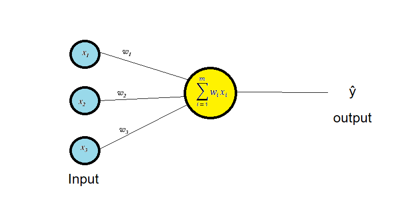
An artificial neural network is a computing system that works like our human brain. (Don’t worry if you don’t know the biological working of our brain.)
ANN is purely mathematical, so don’t bother about it.
Here is an artificial neuron
Let's say you want to predict the chance that you or your friends will go to watch a movie at cinema or not.
Input feature may be like
Whether friends is coming with or not. (Note: 0 denotes No and 1 denotes Yes)
Is cinema hall near.
Whether weather is cool or hot
Weight helps us to know which feature carries, how much importance in decision-making.
Like weights for a guy A who likes friend’s company may be like
w1=5; w2=3; w3=1
And for a guy B who is more concerned about weather condition and distance of cinema hall
w1=2 ; w2= 3; w3=3
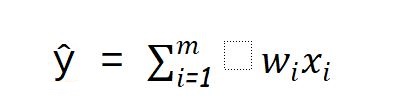
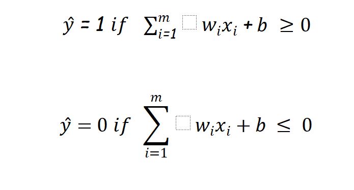
Let us compute our output(whether a person will go to watch movie or not) as :
And let us choose our decision boundary as 5, means a person will go to the cinema hall if Z >= 5.
Then we can conclude based on this condition that
Person A will go if only his friends join him.
Person B will go if friend is with him and cinema hall is near
or
weather is cool and cinema hall is near
We would be able to guess the 3rd condition when B will go.
So we can conclude:
Usually in AI, ML texts this (-5) refers as bias ‘b’ so finally
Finding weights and bias
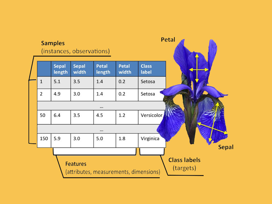
In the practical world we face dataset whose weights are not known to us such that we can correctly classify our target.
Like for the below dataset , to classify flower species we need weights for each feature and a bias.
(NOTE: As above, we discussed 2 class classification and it can be extended to multiclass using more layers.)
So here we will discuss one mostly used technique for finding weights : Gradient descent method
Let we have a dataset containing input features as X = [x1 x2 x3 . . . . xn]
Here :
n = no. of feature
X= input matrix
And target variable as Y.
For Iris dataset we may take x1=sepal length, x2=sepal width ….. and y as class label.
And it will be mostly such that predicted output will get huge value, so we will use activation function such as Sigmoid to overcome it.
Activation Function
There are 3 most commonly used activation function such as:
Rectified Linear Activation (RELU)
Logistic (Sigmoid)
Hyperbolic Tangent (Tanh)
We will discuss Sigmoid in this brief discussion as we go ahead.
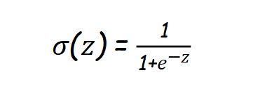
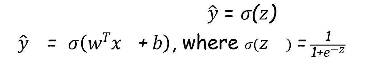
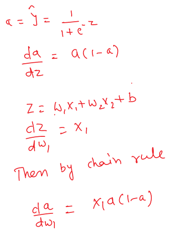
Sigmoid Activation Function
Mathematically
by analyzing above equation we can say that for large value of z , this will return value near to one.
Note:
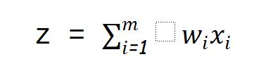
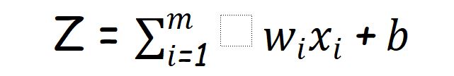
For further use,we will use weighted sum as
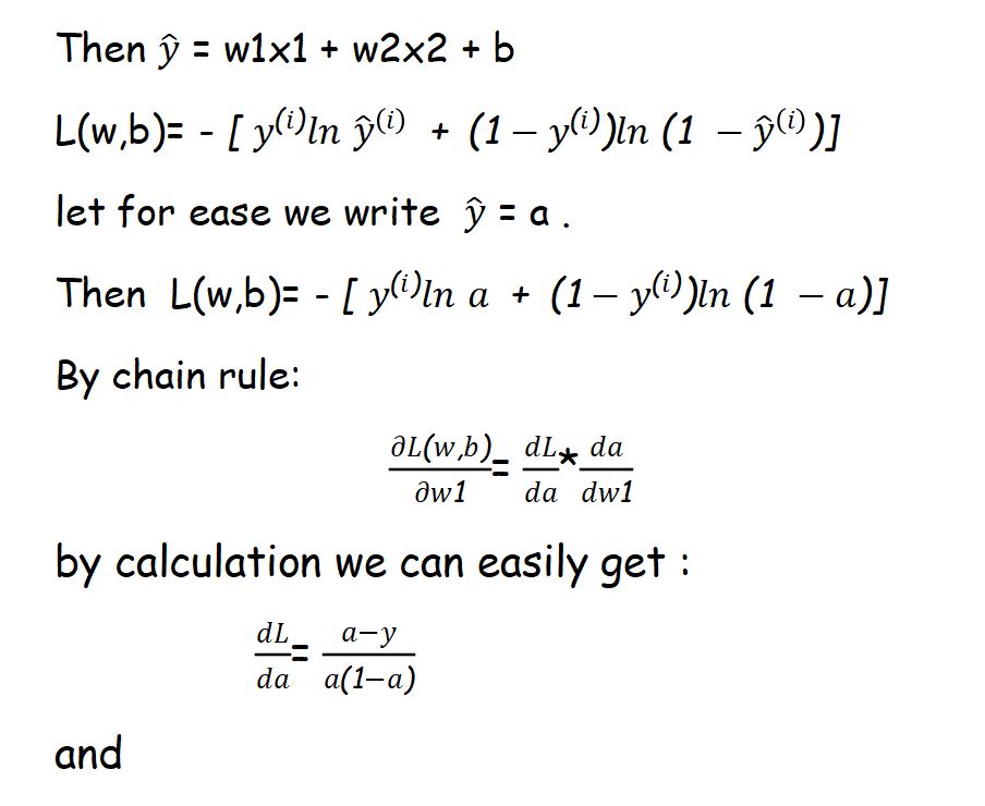
And predicted target variable as
Loss Function
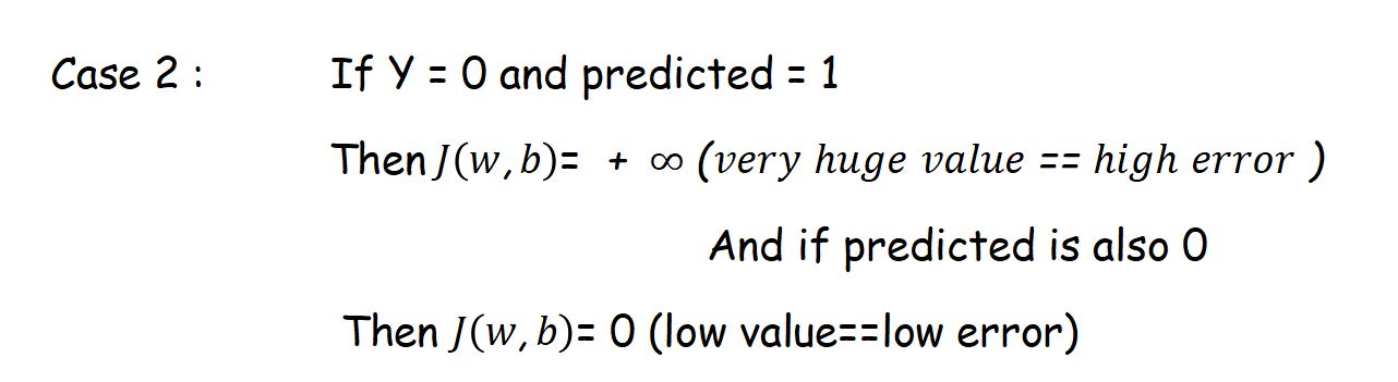
To ensure that our model is going to get correct predicted value or not ,we use LOSS FUNCTION. Loss function measures error between predicted value and actual value.
There are many loss function we use in deep learning.
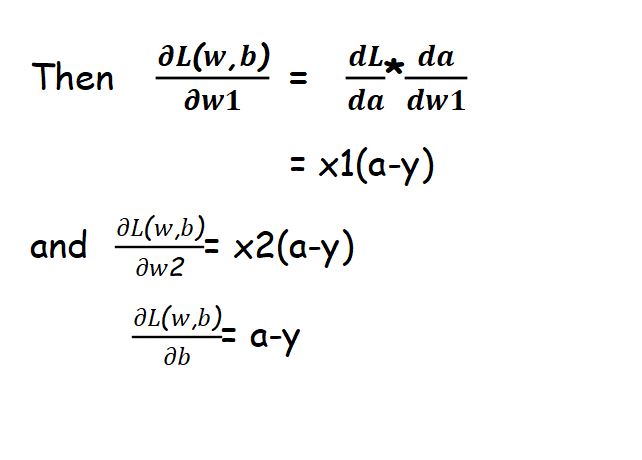
Here we will use cross-entropy loss function J(w,b) described as:
Note : here m = number of inputs.
For understanding let assume
So by above analysis, we can conclude that our goal is to minimize the loss function J(w,b) with proper choice of w and b. This process is called optimization.
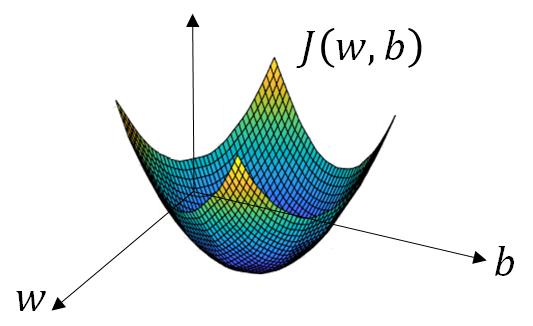
Gradient Descent
One of optimization is Gradient descent which we will discuss here. let suppose our loss function graph looks like below and our goal is to find w , b such it’s value is minimum:
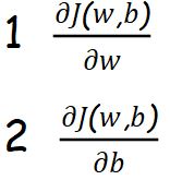
Step 1:
Initialize weights and bias randomly and find
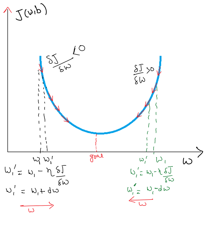
Step 2 :
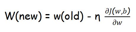
by above graph we can understand that:
and by sufficient number of iteration we get our value of w that will have least error.
we will follow same procedure for finding bias(b).
Step 3:
After finding weight and bias we can simply get our output using these values.
Algorithm
Now we will develop a simple algorithm based on our mathematical understanding:
let we have dataset like below :
X1
X2
Y
0
0
0
0
1
0
1
0
0
1
1
1
So Finally :
import math
x1=[0,0,1,1] #input x1
x2=[0,1,0,1] #input x2
y=[0,0,0,1] #output
w1=0 #initialization of weight and bias
w2=0
b=0
L=0
dw1=0
dw2=0
db=0
for i in range(10000):
a=[]
z=[]
for i in range(4):
z.append(w1*x1[i]+w2*x2[i]+b) #weighted sum
a.append(1/(1+math.exp(-z[i]))) #activation function
L=L+(-(y[i]*math.log(a[i])+(1-y[i])*math.log(1-a[i]))) #Loss function
dz=a[i]-y[i]
dw1=dw1+dz*x1[i] #weight and bias update
dw2=dw2+dz*x2[i]
db=db+dz
dw1=dw1/4
dw2=dw2/4
db=db/4
w1=w1-0.01*dw1
w2=w2-0.01*dw2
b=b-0.01*db
w1 #value of weights after optimization
3.514136610374613
w2
3.514136610374613
b
-5.475789101071454
#testing weight on input
yd=[]
for i in range(4):
yd.append(x1[i]*w1+x2[i]*w2+b)
yd #negative values corresponds to 0 and positive to 1
[-5.475789101071454,
-1.9616524906968413,
-1.9616524906968413,
1.5524841196777714]
Conclusion
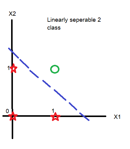
In above discussion we developed a 1 layer neural network with 2 input algorithm purely based on maths and this understanding will help in getting hands on multi-layer neural network.
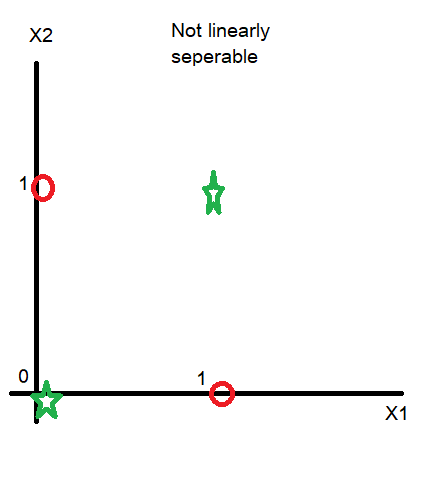
But it have a drawback that it can be applied only on linearly seperable datasets like:
However, with use of Radial basis function we can transform our features from linearly not separable to linearly separable. You can read more about Artificial Neural Networks for Classification.
About the Author's:
Pankaj Singariya
Pankaj Singariya is an ECE final year student of NIT Meghalaya. He loves to learn the mathematical concept behind data science and artificial intelligence and wants to research and work in this field. He has executed projects on data science and machine learning.
Mohan Rai
Mohan Rai is an Alumni of IIM Bangalore , he has completed his MBA from University of Pune and Bachelor of Science (Statistics) from University of Pune. He is a Certified Data Scientist by EMC. Mohan is a learner and has been enriching his experience throughout his career by exposing himself to several opportunities in the capacity of an Advisor, Consultant and a Business Owner. He has more than 18 years’ experience in the field of Analytics and has worked as an Analytics SME on domains ranging from IT, Banking, Construction, Real Estate, Automobile, Component Manufacturing and Retail. His functional scope covers areas including Training, Research, Sales, Market Research, Sales Planning, and Market Strategy.
Table of content
- Motivation
- Introduction
- Finding weights and bias
- Activation function
- Loss function
- Gradient descent
- Algorithm
- Conclusion
We mostly use ready-made deep learning packages such as like Scikit-learn, Keras, TensorFlow etc. and also most of our ML work is easily handled by this.
But for a machine learning practitioner it’s a must to know math and algorithms behind these libraries to get motivation and to stand more in the field.
- It helps us in selecting the right algorithm , right number of parameters, number of features etc.
- AI is in it’s developing phase. Everyday we introduce a number of advancements in it, so mathematical understanding helps us to grasp these techniques.
- It helps us in identifying underfitting and overfitting by Bia_Variance tradeoff.
So here, we will go through some basic math behind artificial neural networks which you will use throughout your learning.
An artificial neural network is a computing system that works like our human brain. (Don’t worry if you don’t know the biological working of our brain.)
ANN is purely mathematical, so don’t bother about it.
Here is an artificial neuron
Let's say you want to predict the chance that you or your friends will go to watch a movie at cinema or not.
Input feature may be like
- Whether friends is coming with or not. (Note: 0 denotes No and 1 denotes Yes)
- Is cinema hall near.
- Whether weather is cool or hot
Weight helps us to know which feature carries, how much importance in decision-making.
Like weights for a guy A who likes friend’s company may be like
w1=5; w2=3; w3=1
And for a guy B who is more concerned about weather condition and distance of cinema hall
w1=2 ; w2= 3; w3=3
Let us compute our output(whether a person will go to watch movie or not) as :
And let us choose our decision boundary as 5, means a person will go to the cinema hall if Z >= 5.
Then we can conclude based on this condition that
- Person A will go if only his friends join him.
- Person B will go if friend is with him and cinema hall is near
or
weather is cool and cinema hall is near
We would be able to guess the 3rd condition when B will go.
So we can conclude:
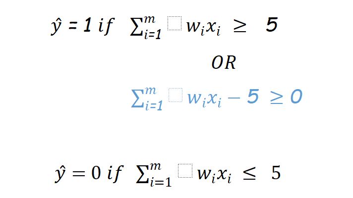
Usually in AI, ML texts this (-5) refers as bias ‘b’ so finally
In the practical world we face dataset whose weights are not known to us such that we can correctly classify our target.
Like for the below dataset , to classify flower species we need weights for each feature and a bias.
(NOTE: As above, we discussed 2 class classification and it can be extended to multiclass using more layers.)
So here we will discuss one mostly used technique for finding weights : Gradient descent method
Let we have a dataset containing input features as X = [x1 x2 x3 . . . . xn]
Here :
n = no. of feature
X= input matrix
And target variable as Y.
For Iris dataset we may take x1=sepal length, x2=sepal width ….. and y as class label.
And it will be mostly such that predicted output will get huge value, so we will use activation function such as Sigmoid to overcome it.
There are 3 most commonly used activation function such as:
- Rectified Linear Activation (RELU)
- Logistic (Sigmoid)
- Hyperbolic Tangent (Tanh)
We will discuss Sigmoid in this brief discussion as we go ahead.
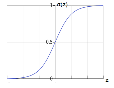
Mathematically
by analyzing above equation we can say that for large value of z , this will return value near to one.
Note:
For further use,we will use weighted sum as
And predicted target variable as
To ensure that our model is going to get correct predicted value or not ,we use LOSS FUNCTION. Loss function measures error between predicted value and actual value.
There are many loss function we use in deep learning.
Here we will use cross-entropy loss function J(w,b) described as:
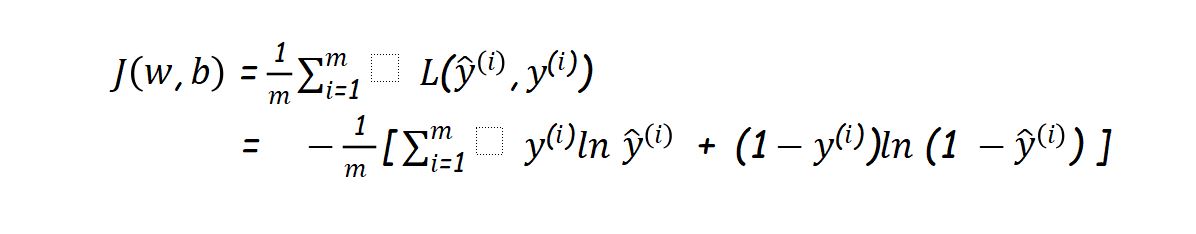
Note : here m = number of inputs.
For understanding let assume
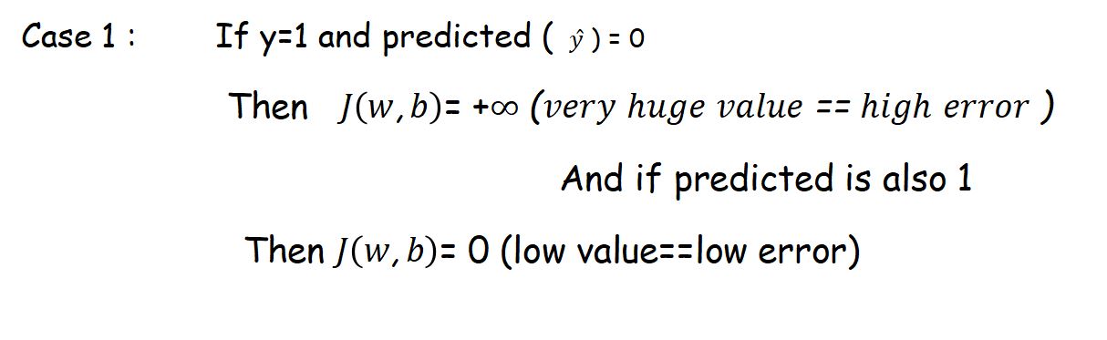
So by above analysis, we can conclude that our goal is to minimize the loss function J(w,b) with proper choice of w and b. This process is called optimization.
One of optimization is Gradient descent which we will discuss here. let suppose our loss function graph looks like below and our goal is to find w , b such it’s value is minimum:
Step 1:
Initialize weights and bias randomly and find
Step 2 :
by above graph we can understand that:
and by sufficient number of iteration we get our value of w that will have least error.
we will follow same procedure for finding bias(b).
Step 3:
After finding weight and bias we can simply get our output using these values.
Now we will develop a simple algorithm based on our mathematical understanding:
let we have dataset like below :
|
X1
|
X2
|
Y
|
|
0
|
0
|
0
|
|
0
|
1
|
0
|
|
1
|
0
|
0
|
|
1
|
1
|
1
|
So Finally :
import math
x1=[0,0,1,1] #input x1
x2=[0,1,0,1] #input x2
y=[0,0,0,1] #output
w1=0 #initialization of weight and bias
w2=0
b=0
L=0
dw1=0
dw2=0
db=0
for i in range(10000):
a=[]
z=[]
for i in range(4):
z.append(w1*x1[i]+w2*x2[i]+b) #weighted sum
a.append(1/(1+math.exp(-z[i]))) #activation function
L=L+(-(y[i]*math.log(a[i])+(1-y[i])*math.log(1-a[i]))) #Loss function
dz=a[i]-y[i]
dw1=dw1+dz*x1[i] #weight and bias update
dw2=dw2+dz*x2[i]
db=db+dz
dw1=dw1/4
dw2=dw2/4
db=db/4
w1=w1-0.01*dw1
w2=w2-0.01*dw2
b=b-0.01*db
w1 #value of weights after optimization
3.514136610374613
w2
3.514136610374613
b
-5.475789101071454
#testing weight on input
yd=[]
for i in range(4):
yd.append(x1[i]*w1+x2[i]*w2+b)
yd #negative values corresponds to 0 and positive to 1
[-5.475789101071454,
-1.9616524906968413,
-1.9616524906968413,
1.5524841196777714]
In above discussion we developed a 1 layer neural network with 2 input algorithm purely based on maths and this understanding will help in getting hands on multi-layer neural network.
But it have a drawback that it can be applied only on linearly seperable datasets like:
However, with use of Radial basis function we can transform our features from linearly not separable to linearly separable. You can read more about Artificial Neural Networks for Classification.
About the Author's:

Write A Public Review