
Table of Content
- Inspiration
- Dataset exploration
- Dependency Packages Installation in your python environment
- Exploratory Data Analysis
- Missing value treatment
- Outlier Treatment
- Feature engineering
- Model Building
- Conclusion
Inspiration
The objective of this project is to identify the presence of diabetes in patient with the help of machine learning (Mathematical complicated calculation, Pun intended). This would help the doctors and insurance companies to save their time and money respectively. I am saying this because to check whether you have diabetes or not you have to go through various tests which may cost you time and money.
Let’s think you have health insurance then they have to bear that cost right. Now if insurance company have some predictive capability to predict the probability of a person having diabetes, it will help them to test only higher probability candidates. This obviously reduces company expenses.
This project is the approach to build that predictive capability using machine learning algorithm by way of automated pipelines. This is an end to end project.
Dataset exploration
First step in ML project is to understand the problem and dataset. Here the datasets we will be using consists of several medical variables (features) and one target variable (Outcome).
- Pregnancy: This indicates number of times a female subject was pregnant
- Glucose: Glucose concentration a 2 hour in an oral glucose tolerance test (mg/dl) - A 2-hour value between 140 and 200 mg/dL (7.8 and 11.1 mmol/L) is called impaired glucose tolerance. This is called "pre- diabetes." It means you are at increased risk of developing diabetes over time. A glucose level of 200 mg/dL (11.1 mmol/L) or higher is used to diagnose diabetes.
- BloodPressure: Diastolic blood pressure (mm Hg)- If Diastolic B.P > 90 means High B.P (High Probability of Diabetes) Diastolic B.P < 60 means low B.P (Less Probability of Diabetes)
- Skin Thickness: Triceps skinfold thickness (mm) -A value used to estimate body fat. Normal Triceps SkinFold Thickness in women is 23mm. Higher thickness leads to obesity and chances of diabetes increases.
- Insulin: 2-Hour Serum Insulin (mu U/ml) - Normal Insulin Level 16-166 mIU/L Values above this range can be alarming.
- BMI: Body Mass Index (weight in kg/ height in m2) - Body Mass Index of 18.5 to 25 is within the normal range BMI between 25 and 30 then it falls within the overweight range. A BMI of 30 or over falls within the obese range.
- DiabetesPedigreeFunction: It provides information about diabetes history in relatives and genetic relationship of those relatives with patients. Higher Pedigree Function means patient is more likely to have diabetes.
- Age: Age in years
- Outcome: Class variable (either 0 or 1)- where ‘0’ denotes having diabetes and ‘1’ denotes patient having diabetes The dependent variable is whether the patient is having diabetes or not.
Dependency Packages Installation in your python environment
We will install packages in python by using “pip” followed by install package name. For example, write “ pip install sklearn ” and run that tab when you are using jupyter notebook.
Required packages are as below:
- Pandas- to perform dataframe operations
- Numpy- to perform array operations
- Matplotlib- to plot charts
- Seaborn – to plot charts
- Missingo- anlysing the missing values
- sklearn – to build the model
- pickle- to save and load the model
Loading the libraries and dataset
    # import required libraries
    import pandas as pds
    import numpy as np
    import matplotlib.pyplot as plot
    import seaborn as sn
    %matplotlib inline
    import warnings
    warnings.filterwarnings('ignore')
    import missingno as msno
Download the Diabetic data set by clicking here.
    # Loading the dataset( Assumption : data file is in working directory )
    diabetes_df=pds.read_csv('health_care_diabetes.csv')
Exploratory Data Analysis
For classification problems we need a balanced data set. We will check imbalance in our data by using value_counts function which in turn counts the rows of each class in one column.
    # Check if the data is a Balanced one or not
    print(diabetes_df.Outcome.value_counts())
    diabetes_df.Outcome.value_counts().plot(kind='barh')
0 500
1 268
Name: Outcome, dtype: int64
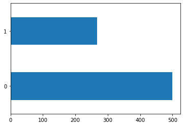
Figure 1 : Distribution of the target variable (Diabetic - Yes/No) to confirm unbalanced data set problem
Key observations from figure 1,
- we got an imbalanced dataset
    # Compute basic statistic for our data
    # Columns with non-numerical data would be not be displayed unless we specify the parameter include="all"

    #transpose the result use '.T'
    diabetes_df.describe().T
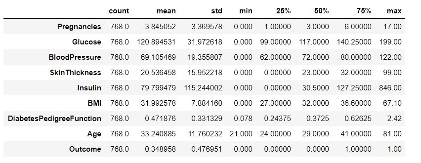
Figure 2 : Descriptive Statistics for the Diabetic data set
Key observations from figure 2,
- After looking at the mean, median and mode along with the histogram we can say that most of features are skewed just because of the zero values concentration on one side, and having some outliers
- On following columns, zero does not make sense and indicates presence of missing value.
- Glucose
- BloodPressure
- SkinThickness
- Insulin
- BMI
- As total observation are 768, so for now we can say there is no missing values.
Recommended to replace zero values with NaN for better understanding and interpretation of dataset.
Missing value treatment
    # making a copy of dataframe
    df_copy = diabetes_df.copy(deep = True)
    #replace zero values as nan in relevent columns
    for i in df_copy[['Glucose', 'BloodPressure', 'SkinThickness', 'Insulin', 'BMI']]:
        df_copy[i].replace(0, np.nan, inplace= True)

    # we will plot missing matrix map with missingno package
    msno.bar(df_copy, figsize=(8,6),fontsize=10)
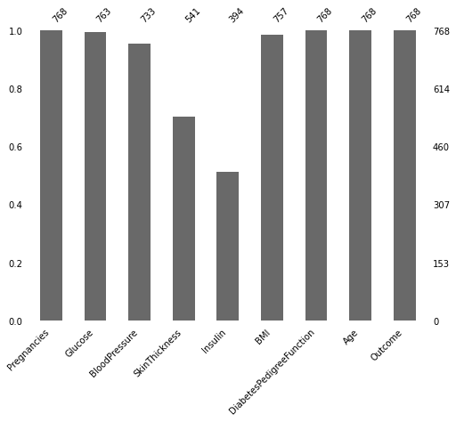
Figure 3 : Identifying the missing values in the data by looking at the count distribution
Now we know there are so many missing values. There are two ways to handle this issue, we can delete the whole row containing missing value or deleting the whole column if missing value percentage is more than 60%. Here in this dataset we got missing values in insulin column but we know that for predicting diabetes insulin is best feature thus we will keep all the features as it is and we will impute missing values by using mean value of that column.
    # split data in two dataframes based on Outcome to impute NaN values
    df1=df_copy[(df_copy.Outcome==0)]
    df2=df_copy[(df_copy.Outcome==1)]
    df1.fillna(df1.mean(),inplace=True)
    df2.fillna(df2.mean(),inplace=True)

    df_copy1=pds.concat((df1,df2),axis=0)
    df_copy1.sort_values(by='Age',inplace=True)
    df_copy1.reset_index(drop=True,inplace=True)
    df_copy1.isna().sum()
Pregnancies 0
Glucose 0
BloodPressure 0
SkinThickness 0
Insulin 0
BMI 0
DiabetesPedigreeFunction 0
Age 0
Outcome 0
dtype: int64
we have successfully imputed the missing values.
Outlier Treatment
We will plot boxplot to analyse and understand the extreme values , so that we can better understand how many values are out of the interquartile range and which features are having more number of outliers.
    # Outliers Visualization
    def plot_outliers(df):
        df_name = df.columns
        fig, axs = plot.subplots(1, len(df_name), figsize=(20, 10))

        for i, col in enumerate(df_name):
            axs[i].set_title(col)
            axs[i].boxplot(df[col])
        fig.suptitle('Outliers');

    plot_outliers(df_copy1)
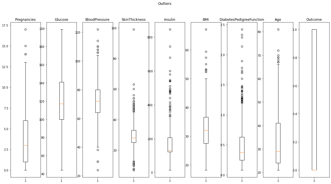
Figure 4 : Checking the outliers in diabetics data using box plots
What to do with these outliers
From above boxplot and function output we came to know that there are some outliers which are very extreme values.
- Outliers are having some useful information or they are just because of typo error. we will verify it by removing extreme values at first....If accuracy not achieved then we will drop all outlier's.
- Insulin and DiabetesPedigreefunction having many outlier's. so we will remove only extreme values just to avoid data loss.
Note:
- Outliers leads to make wrong decisions by making wrong if else loop in decesion trees whenever outlier is a typo and also its not easy for liniear methods to handle outliers.
But when it is genuine and containing useful information at that time droping it will loss of information. In short model will not be able to be generalised.
    # Insulin value above 420 are extreme and making tail longer so we will drop them
    df_copy1=df_copy1[(df_copy1.Insulin<=420)]

    # skinthickness above 80 has only one datapoint so we will drop it
    df_copy1=df_copy1[(df_copy1.SkinThickness<=80)]

    # Blood Pressure below 20 doesn't make sense so we will drop it
    df_copy1=df_copy1[(df_copy1.BloodPressure>=20)]

    # BMI above 60 has only one datapoint so we will drop it
    df_copy1=df_copy1[(df_copy1.BMI<=60)]

    # DiabetesPedigreeFunction value above 2 are extreme and making tail longer so we will drop them
    df_copy1=df_copy1[(df_copy1.DiabetesPedigreeFunction<=2)]

    # Age value above 80 are extreme and making tail longer so we will drop them
    df_copy1=df_copy1[(df_copy1.Age<=80)]

    # Pregnancies value above 15 are extreme and making tail longer so we will drop them
    df_copy1=df_copy1[(df_copy1.Pregnancies<=15)]
    df_clean=df_copy1.copy(deep=True)

    # dataframe shape before and after outlier treatment
    print('Before outlier removal dataset shape is', df_copy.shape)
    print('After outlier removal dataset shape is', df_copy1.shape)
Before outlier removal dataset shape is (768, 9)
After outlier removal dataset shape is (744, 9)
We have successfully removed those extreme values from the dataset which may have created more noise to build a model, resulting in lower score.
Further we will do some feature engineering and EDA to better understand the features and creating newer ones.
Feature engineering
We will further analyse the dataset distribution using pairplot method available in seaborn.
    # pairplot
    sn.pairplot(df_clean, hue='Outcome')
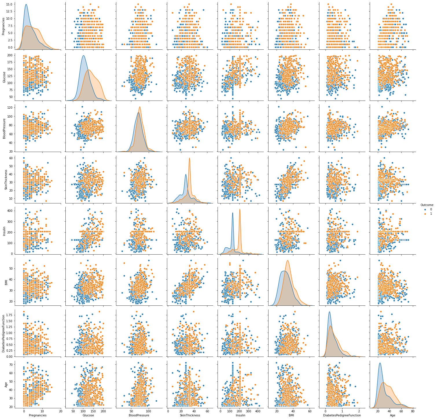
Figure 5 : Look at the distribution of diabetic data using pairplot in seaborn
    # close look on scatter plot of Glucose vs Age which seems to be corelated
    sn.scatterplot(x = df_clean['Glucose'], y = df_clean['Age'], hue = "Outcome", data = df_clean)
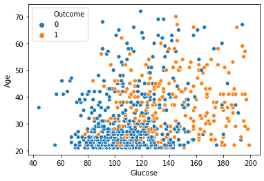
Figure 6 : Scatter plot of glucose and age highlights the correlation
Observations :
- From above pairplot diagonal KDE plot we can conclude that our clean data looks normally distributed. Except Pregnancies and Age and DiabetesPedigreeFunction these features slightly right skewed
- Scatterplots showing data points are not easily linearly separable as they are overlapped, thus linear classification algorithms will not be able to give higher accuracy.
- Pairplot shows 'BloodPressure' and 'DiabetesPedigreeFunction' has similar KDE distribution for both Outcomes so it might not suitable for separation
- Glucose has close relation with insulin and Age and most of healthy peopels found within a range of Glucose 40 to 120 and data is more concentrated there, Over this Glucose range we can predict most probably the person is Diabetic
we will create new features depending on what we come to know from our EDA
    df_clean['AG_Prob_D']= np.where(((df_clean.Glucose<=150) & (df_clean.Age<30)),0,1)

    df_clean['IG_Prob_D']= np.where(((df_clean.Insulin<=150)&(df_clean.Glucose<=130)),0,1)

    df_clean['Preg_DPF']= df_clean.DiabetesPedigreeFunction*df_clean.Pregnancies
Correlation Heatmap
    # correlation of features
    corr=df_clean.corr()
    sn.heatmap(corr[(corr >= 0.2) & (corr >= -0.2)],annot=True)
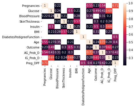
Figure 7 : Correlation grid for diabetic data set
Observations:
- DiabetesPedigreeFunction and Blood pressure has no linear corelation with outcome more than 0.2. So these variables will not be helpful with linear classification models
- No feature is highly corelated with outcome. Insulin, Glucose and newly created features are having slightly higher corelation with outcome.
Model Building
Train Test Split (Hold Out Method) : A mechanism of identifying the train and test data splits, usually a 2/3 blocked splits. If there is surety of absence of bias-variance anomaly, then the modeller can decide whether he want's a 70:30 split or 70:20:10 split. In certain cases, we may go for 50:50, specifically when we expect over learning by the model.
Cross Validation: Instead of segmenting the data into train, test and validation sets, or train test splits, we can get equal sized blocks called as folds. As a programmer, you can decide, if you want 3/5/7... folds. One of the folds will be the test set and the other combined would be the train set. There are many variations within this adding randomness vs sequential.
Stratify : Stratify parameter makes sure that the number of cases in the population data is maintained in the same proportion in the split data sets.
    # Its always recommended to set a seed for reproducibility, so that you can simulate the same sets for experimenation and rectification of models
    SEED = 10

    # converting and splitting  features and label into numpy array train and test data
    from sklearn.model_selection import train_test_split
    features, label = df_clean.iloc[:,[1,2,3,4,5,7,9,10,11]],df_clean.iloc[:,[8]]

    # train, test split(we will be validate our model on 20?ta with test cases and will build model with CV)

    X_train, X_test, y_train, y_test = train_test_split(features, label, test_size=0.2, random_state=SEED,stratify=label)
What is Imbalanced Dataset
In order to make our dataset Balanced we will use imblearn package. With the help of oversampling we will get a balanced dataset for modeling so that our model will not tends towards predicting more zero class rather than one class for which we are interested.
Note: we are considering that we are focused to classify correctly the Diabetic(outcome=1) person. (If both outcomes have same weight then there is no need of oversampling.)
    print("Before Over Sampling, counts: Features {} and Label {}".format(X_train.shape,y_train.shape))
    print("{}".format(y_train.Outcome.value_counts()))
    # import SMOTE module from imblearn library
    # Because of permission, installing from package managers like Anaconda Navigator may not work
    # Hence use Anaconda prompt or command prompt or terminal
    # pip install -U imbalanced-learn
    from imblearn.over_sampling import SMOTE
    sm = SMOTE(random_state = 64)
    X_train_os, y_train_os = sm.fit_resample(X_train, y_train)

    print("After Over Sampling, counts: Features {} and Label {}".format(X_train_os.shape,y_train_os.shape))
    print("{}".format(y_train_os.Outcome.value_counts()))
Before Over Sampling, counts: Features (595, 9) and Label (595, 1)
0 394
1 201
Name: Outcome, dtype: int64
After Over Sampling, counts: Features (788, 9) and Label (788, 1)
1 394
0 394
Name: Outcome, dtype: int64
Build the Machine Learning Model
To build an efficient model, we need to compare the performance of various machine learning classification algorithms. So that we can achieve best F1 score. F1 score is the harmonic mean of recall and precision.
    from sklearn.pipeline import Pipeline
    from sklearn.preprocessing import StandardScaler
    from sklearn.model_selection import cross_validate, cross_val_score,ShuffleSplit
    from sklearn.metrics import accuracy_score, confusion_matrix ,classification_report,roc_auc_score,auc
    from sklearn.svm import SVC
    from sklearn.linear_model import LogisticRegression
    from sklearn.ensemble import RandomForestClassifier, GradientBoostingClassifier
    from sklearn.neighbors import KNeighborsClassifier

    cv_split = ShuffleSplit(n_splits = 10, test_size = 0.1, train_size = 0.9, random_state = 0)
    pipeline = Pipeline([
        ('scale', StandardScaler()), # Step1 - normalize data
        ('clf', LogisticRegression()) # Step2 - classifier
    ])
    pipeline.steps


    clfs = []
    clfs.append(LogisticRegression())
    clfs.append(SVC())
    clfs.append(KNeighborsClassifier(n_neighbors=5))
    clfs.append(RandomForestClassifier(max_depth=6))
    clfs.append(GradientBoostingClassifier(n_estimators=100))

    results=[]
    results1=[]
    results2=[]
    results3=[]
    for classifier in clfs:
        pipeline.set_params(clf = classifier)
        scores = cross_validate(pipeline, X_train, y_train, cv=cv_split, return_train_score=True)
        # default parameter fit for comparision with CV Score and Default fit score
        pipeline.set_params(clf = classifier)
        pipeline.fit(X_train,y_train)
        train_acc=pipeline.score(X_train, y_train)
        test_acc=pipeline.score(X_test, y_test)
        print('---------------------------------')
        print(str(classifier))
        print('-----------------------------------')
        for key, values in scores.items():
                if key=='test_score':
                    results.append({'Test_mean_Score': values.mean(), 'Test_Std': values.std()})
        for key, values in scores.items():
                if key=='train_score':
                    results1.append({'Train_mean_Score': values.mean(), 'Train_Std': values.std()})
        for key, values in scores.items():
                if key=='fit_time':
                    results2.append({'Fit_time': values.mean()})

        results3.append({'Def_Train_score':train_acc,'Def_Test_score':test_acc})
    results=pds.DataFrame(results,index=['LR','SVC','KNN','RF','GB'])
    results1=pds.DataFrame(results1,index=['LR','SVC','KNN','RF','GB'])
    results2=pds.DataFrame(results2,index=['LR','SVC','KNN','RF','GB'])
    results3=pds.DataFrame(results3,index= ['LR','SVC','KNN','RF','GB'])

    Compare_models=pds.concat((results,results1,results3,results2),axis=1)
    Compare_models.sort_values(by='Test_mean_Score',ascending=False)
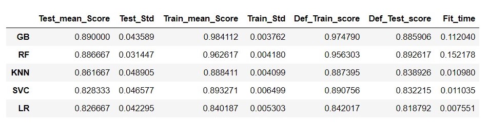
Figure 8 : Evaluation Metrics of models created using ML Pipelines
From figure 8, it is clear that Gradient Boosting model is performing very well with cross validation and with default setting also, so we will go with hyper tuning for Gradient Boosting model.
Hyper Tuning for Gradient Boosted Algorithm
    from sklearn.model_selection import RandomizedSearchCV
    pipeline.set_params(clf= GradientBoostingClassifier())
    pipeline.steps

    param_grid = {
        'clf__loss' : ['deviance', 'exponential'],
        'clf__n_estimators' : [20,35,55,75,85,95],
        'clf__random_state': np.arange(1,50),
        'clf__max_depth': [3,4,5,6,7,8,10]
    }

    gbm_grid = RandomizedSearchCV(pipeline,param_grid, cv=cv_split, n_iter = 10 )
    gbm_grid.fit(X_train, y_train)
    gbm_grid=gbm_grid.best_estimator_
    gbm_grid
    y_predict = gbm_grid.predict(X_test)
    y_prob= gbm_grid.predict_proba(X_test)
    accuracy = accuracy_score(y_test,y_predict)
    print(accuracy)
    print('auc=', roc_auc_score(y_test,y_prob[:,1]))

    print(classification_report(y_test,y_predict))
    confusion_matrix(y_test,y_predict)
0.8859060402684564
auc= 0.9648484848484848
precision recall f1-score support
0 0.94 0.89 0.91 99
1 0.80 0.88 0.84 50
accuracy 0.89 149
macro avg 0.87 0.88 0.88 149
weighted avg 0.89 0.89 0.89 149
array([[88, 11],
[ 6, 44]], dtype=int64)
In our final output we got F1 score of 84% for class 1 and 91% for class 0. This is pretty good score and we can go further to use this model by saving the model using pickle library as below:
    import pickle

    pickle.dump(gbm_grid, open("diabetes.pickle.dat", "wb"))
we can reuse this model again and again by using below code.
    model=pickle.load(open("diabetes.pickle.dat", "rb"))
    model
Conclusion
Automated pipelines are used exhaustively in product development wherein organizations offer cloud services for Auto ML. What we saw in this blog was an implementation on a pretty generic and exhausively used ML dataset - Diabetics data set. You should first execute this program once interpreting the details as you execute. Once done, I would suggest using a different data set and see, if it works for you. Although we have used pipelines for model selection, when it comes to hyper parameter tuning, we have again gone manual. As a next step, you can try automating that part by used of pipelines and user defined function. In some other blog, I would cover that as well. Do comment and let me know your inputs and any challenges faced while implementing this end to end project. Recommend you to read this blog on Machine learning using only Numpy.
About the Author:
Write A Public Review