
Table of Content
- Introduction
- Imbalance classes vs Unbalanced classes
- Types of Imbalance
- Why it is important to handle imbalance data
- How to handle imbalance data
- Performing class balancing on Telecom Churn Dataset
- Conclusion
Introduction
Imbalanced Classes, is the condition in which one type of class/data is more than the other type of data. It means that the data is skewed toward a particular type of class and favors the results of the machine learning model for that class.
It is observed in classification problems only as the target variable value is discrete. It not only affects binary classification but also greatly affects the multiclass classification problem.
Example- Suppose we are working on a dog cat classifier and we have a dataset that has only 20% dog flags and 80?t flags. This dataset is thus known as imbalanced data and the classes are imbalanced classes.
Imbalance classes vs Unbalanced classes
Now the question arises – What is the difference between imbalance classes and unbalanced classes? So the answer to this question lies in the definition of these two classes, as we already know the definition of imbalance class we will now understand what is unbalanced classes. An unbalanced class refers to that class that was balanced at an early stage but now it is not balanced either due to preprocessing or splitting of the dataset.
Example of Imbalanced Classes:
Suppose you have 10 candies of 2 flavors – mango and orange. If you have 4 candies of mango flavor and 6 candies of orange flavor. This is the case of imbalance classes as the number of mango-flavored candy is less than orange-flavored candy.
Example of Unbalanced Classes:
Suppose you have 10 candies of 2 flavors – mango and orange. Now you have the same number of candies for both the flavors but for training and testing you took 4 mango-flavored candy and 3 orange-flavored candy now even though the data was balanced initially but due to splitting the data becomes unbalanced.
Types of Imbalance
Classification of imbalance in classes is based on the percent or how much the actual difference is there between the classes and based on that difference we define the imbalance.
Slight Imbalance - This is the imbalance in which the data difference between the classes is non-significant or not much. The general 40% to 60 % coverage of classes comes under this category.
Severe Imbalance - This is the imbalance in which the data difference between the classes is significant. The general 70% to 99 % coverage of classes comes under this category.
Why it is important to handle imbalance data
The main reason we try to remove the imbalance between the classes is that it greatly affects the accuracy of our model. Now the question arises why is it so? And the answer lies like machine learning algorithms that are whenever any event occurs non frequently it is considered as a rare event. The standard machine learning classification algorithm has a bias toward those classes that have a large number of values. Hence the classes having fewer data are treated as noise and are often ignored causing to predict only those classes as a result which are large in number. This generally gives high accuracy results but fails to perform well on the F-1 score.
How to handle imbalance data
Using data resampling techniques
This is the data level approach in which we perform resampling of data to balance the number of values for each class.
Random Under Sampling
In this type of sampling technique, the class consist of more data is considered and a percentage of its data is only taken for the algorithm to balance the class size.
But this type of sampling causes a huge loss of data and hence some way may affect the full potential of the model.
Random Over Sampling
In this type of sampling technique, the class consist of less data is considered and the data of this class is replicated to reduce the gap between the size of majority and minority class.
But this type of sampling causes the overfitting of data as there is huge redundancy in the dataset.
SMOTE(Synthetic Minority Oversampling Technique)
This is the technique that is used to avoid overfitting that is caused by random oversampling as the data is a replica of the same data. This method takes the subset of the data and then creates the synthetic instances of the data. These synthetic instances are different from the original data and are added to the original dataset. The new dataset thus obtained is used as a sample to train the classification models.
But it is ineffective for high dimensional data.
Using algorithmic ensembling technique
In this, we use external algorithms to resample the class data.
Bagging Based Balancing Method
In this, the data is divided into different parts and each part is different from the dataset and at last, the final result is obtained from the aggregated values from every output obtain from each part of the data.
Boosting Based Balancing Method
It uses two boosting methods that are Ada Boost method and the Gradient Tree Boosting method to perform the Balancing of classes. The basic intuition of this method is that it combines base/weak classifiers that give average outcomes to the strong learners.
Performing class balancing on Telecom Churn Dataset
    # importing the necessary libraries
    import numpy as np
    import pandas as pd
    import matplotlib.pyplot as plt
    import seaborn as sns
    import imblearn
    from sklearn.linear_model import LogisticRegression
    from sklearn.preprocessing import OneHotEncoder
    from sklearn.metrics import confusion_matrix
    from sklearn.metrics import classification_report
    from sklearn.model_selection import train_test_split
    from sklearn.metrics import accuracy_score
    from imblearn.under_sampling import RandomUnderSampler
    from imblearn.over_sampling import RandomOverSampler
    from imblearn.combine import SMOTETomek
    import warnings
    warnings.filterwarnings('ignore')

    # Reading the csv data and checking the columns
    # Download the churn data from this link
    data = pd.read_csv("churn-data.csv")
    data.columns
Index(['customerID', 'gender', 'SeniorCitizen', 'Partner', 'Dependents',
       'tenure', 'PhoneService', 'MultipleLines', 'InternetService',
       'OnlineSecurity', 'OnlineBackup', 'DeviceProtection', 'TechSupport',
       'StreamingTV', 'StreamingMovies', 'Contract', 'PaperlessBilling',
       'PaymentMethod', 'MonthlyCharges', 'TotalCharges', 'Churn'],
      dtype='object')
    # Giving first glance to the data
    pd.set_option('display.max_columns', None)
    data.head()

   customerID  gender  SeniorCitizen Partner Dependents  tenure PhoneService     MultipleLines InternetService OnlineSecurity OnlineBackup DeviceProtection TechSupport StreamingTV StreamingMovies        Contract PaperlessBilling              PaymentMethod  MonthlyCharges TotalCharges Churn
0  7590-VHVEG  Female              0     Yes         No       1           No  No phone service             DSL             No          Yes               No          No          No              No  Month-to-month              Yes           Electronic check           29.85        29.85    No
1  5575-GNVDE    Male              0      No         No      34          Yes                No             DSL            Yes           No              Yes          No          No              No        One year               No               Mailed check           56.95       1889.5    No
2  3668-QPYBK    Male              0      No         No       2          Yes                No             DSL            Yes          Yes               No          No          No              No  Month-to-month              Yes               Mailed check           53.85       108.15   Yes
3  7795-CFOCW    Male              0      No         No      45           No  No phone service             DSL            Yes           No              Yes         Yes          No              No        One year               No  Bank transfer (automatic)           42.30      1840.75    No
4  9237-HQITU  Female              0      No         No       2          Yes                No     Fiber optic             No           No               No          No          No              No  Month-to-month              Yes           Electronic check           70.70       151.65   Yes
    # Getting information of the columns
    data.info()

RangeIndex: 7043 entries, 0 to 7042
Data columns (total 21 columns):
 #   Column            Non-Null Count  Dtype
---  ------            --------------  -----
 0   customerID        7043 non-null   object
 1   gender            7043 non-null   object
 2   SeniorCitizen     7043 non-null   int64
 3   Partner           7043 non-null   object
 4   Dependents        7043 non-null   object
 5   tenure            7043 non-null   int64
 6   PhoneService      7043 non-null   object
 7   MultipleLines     7043 non-null   object
 8   InternetService   7043 non-null   object
 9   OnlineSecurity    7043 non-null   object
 10  OnlineBackup      7043 non-null   object
 11  DeviceProtection  7043 non-null   object
 12  TechSupport       7043 non-null   object
 13  StreamingTV       7043 non-null   object
 14  StreamingMovies   7043 non-null   object
 15  Contract          7043 non-null   object
 16  PaperlessBilling  7043 non-null   object
 17  PaymentMethod     7043 non-null   object
 18  MonthlyCharges    7043 non-null   float64
 19  TotalCharges      7043 non-null   object
 20  Churn             7043 non-null   object
dtypes: float64(1), int64(2), object(18)
memory usage: 1.1+ MB
    # Checking how much difference is there in the target variables
    x = np.array(data["Churn"].unique())
    y = np.array(data["Churn"].value_counts())
    sns.barplot(x=x,y=y)
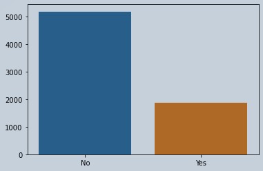
Figure 1 : Visual representation of imbalanced data set
    # This function is for encoding data which is in Yes and No format
    def encodingforYes(series):
        if series=="No":
            return 1
        else:
            return 0

    def encodingforgender(series):
        if series=="Male":
            return 1
        else:
            return 0
    # Columns that consist of data in yes and no format
    columns = ['Partner','Dependents','PhoneService', 'OnlineSecurity', 'OnlineBackup', 'DeviceProtection'
             ,'TechSupport', 'StreamingTV', 'StreamingMovies','PaperlessBilling','Churn']

    # Traversing on the columns list and applying the encoding function
    for i in columns:
        data[i] = data[i].apply(encodingforYes)

    data['gender']=data['gender'].apply(encodingforgender)
    # Function so as to perform onehot encoding on the categorical data
    def onehot(column):
        heading = column.unique()
        newheading = [i+str(column) for i in heading]
        data = OneHotEncoder(sparse=False).fit_transform(np.array(column).reshape(-1,1))
        subframe = pd.DataFrame(data,columns=newheading)
        return subframe

    # Traversing on the categorical columns
    onehotcolumns=['MultipleLines','InternetService','Contract','PaymentMethod']

    for i in onehotcolumns:
        column = data[i]
        data.drop(i,axis=1,inplace=True,)
        frame = onehot(column)
        data = pd.concat([data,frame],axis=1)
    # Converting object type data into numeric type as Logistic Regression don't understand object data
    def conversion(value):
        if(value==" "):
            return '0'
        else:
            return value
    data['TotalCharges'] = data['TotalCharges'].apply(conversion)
    data['TotalCharges'] = pd.to_numeric(data['TotalCharges'])

    # Dropping unwanted column
    data.drop("customerID",axis=1,inplace=True)
    len(data.columns)

29

    # Initializing a Simple LogisticRegression object
    lr = LogisticRegression()

    # Distributing data in terms of independent and dependent variables
    X = data.drop('Churn',axis=1)
    y = data['Churn']

    # Splitting data in train and test
    X_train,X_test,y_train,y_test = train_test_split(X,y,test_size=0.3)

    # Fitting data
    lr.fit(X_train,y_train)

    # Predicting the data
    y_pred = lr.predict(X_test)

    # Checking the precision, recall, f1-score and accuracy
    print(classification_report(y_pred,y_test))

              precision    recall  f1-score   support

           0       0.56      0.66      0.60       470
           1       0.90      0.85      0.87      1643

    accuracy                           0.81      2113
   macro avg       0.73      0.75      0.74      2113
weighted avg       0.82      0.81      0.81      2113
    # Now performing undersampling on the data with sampling strategy 1 which means data of both classes will be same
    undersampler = RandomUnderSampler(sampling_strategy=1)

    X_under,y_under = undersampler.fit_resample(X,y)


    y_ = np.array(y_under.value_counts())
    sns.barplot(x=x,y=y_)
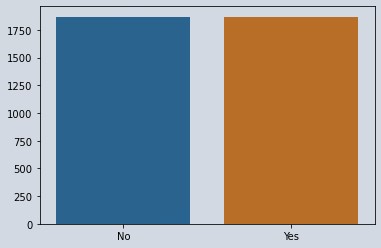
Figure 2 : Balanced Data Using Under Sampling
    print(y_under.value_counts())

1    1869
0    1869
Name: Churn, dtype: int64
    X_under_train,X_under_test,y_under_train,y_under_test = train_test_split(X_under,y_under,test_size=0.3)
    lr.fit(X_under_train,y_under_train)
    y_under_pred = lr.predict(X_under_test)
    print(classification_report(y_under_pred,y_under_test))

              precision    recall  f1-score   support

           0       0.80      0.72      0.76       608
           1       0.71      0.79      0.75       514

    accuracy                           0.75      1122
   macro avg       0.76      0.76      0.75      1122
weighted avg       0.76      0.75      0.75      1122
Now you can see after performing undersampling our score reduced as we lost some information.
    # Now performing oversampling on the data with sampling strategy 1 which means data of both classes will be same
    oversampler = RandomOverSampler(sampling_strategy=1)

    X_over,y_over = oversampler.fit_resample(X,y)


    y_ = np.array(y_over.value_counts())
    sns.barplot(x=x,y=y_)
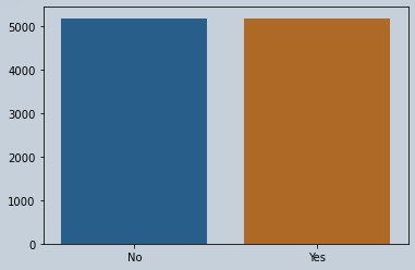
Figure 3 : Balanced Data Using Over Sampling
    print(y_over.value_counts())

1    5174
0    5174
Name: Churn, dtype: int64
    X_over_train,X_over_test,y_over_train,y_over_test = train_test_split(X_over,y_over,test_size=0.3)
    lr.fit(X_over_train,y_over_train)
    y_over_pred = lr.predict(X_over_test)
    print(classification_report(y_over_pred,y_over_test))

              precision    recall  f1-score   support

           0       0.81      0.75      0.78      1670
           1       0.73      0.79      0.76      1435

    accuracy                           0.77      3105
   macro avg       0.77      0.77      0.77      3105
weighted avg       0.77      0.77      0.77      3105
Now you can see after performing oversampling our score reduced as the data redundancy increased causing overfitting.
    # Now performing oversampling using SMOTETomek on the data with sampling strategy 1 which means data of both classes will be same
    smote = SMOTETomek(sampling_strategy=1)

    X_smote,y_smote = smote.fit_resample(X,y)

    y__ = np.array(y_smote.value_counts())
    sns.barplot(x=x,y=y__)
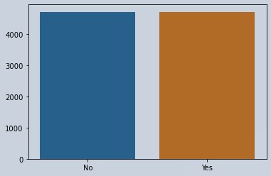
Figure 3 : Balanced Data Using Over Sampling using SMOTETomek
    print(y_smote.value_counts())

1    4724
0    4724
Name: Churn, dtype: int64

X_smote_train,X_smote_test,y_smote_train,y_smote_test = train_test_split(X_smote,y_smote,test_size=0.3)
lr.fit(X_smote_train,y_smote_train)
y_smote_pred = lr.predict(X_smote_test)
print(classification_report(y_smote_pred,y_smote_test))

              precision    recall  f1-score   support

           0       0.81      0.79      0.80      1455
           1       0.79      0.80      0.80      1401

    accuracy                           0.80      2856
   macro avg       0.80      0.80      0.80      2856
weighted avg       0.80      0.80      0.80      2856
Now you can see after performing oversampling by SMOTETomek our score increased as the data formed is different than the original data.
Conclusion
Whenever any dataset contains any imbalanced classes then, we can’t directly rely on our machine learning models accuracy metrics as the output is generally skewed toward the majority class. It is very important to perform data sampling. You should also read through this article on Cross Vaidation in ML Models. This will help you with techniques for validating the models.
About the Author's:
Write A Public Review