
Decision Tree in a Nutshell Using Python
Table of Content
Introduction
Terms used in Decision Tree
Types of Decision Tree
Working of Decision Tree in Machine Learning
Advantaged of Decision Tree
Disadvantages of Decision Tree
Application of Decision Tree
Creating Decision Tree from basics using Python
Import all the Libraries
Load DataSet
Exploratory Data Analysis
Data Set Preparation
Build the Decision tree model
Use the models to predict the data in test environment
Conclusion and Summary
Decision Tree
Decision tree is a predictive model which is widely used in machine learning. In decision tree, the given data is continuously divided based on the given input. It is a supervised machine learning technique in which the data is divided into nodes and leaves similar to a tree, in which nodes are the input(question) and leaves are the output(answer). Mostly it starts with single node which gets divided into possible outcome. It is used in statistics and data mining to solve classification or regression problem in the form of tree. It is very effective for non-linear dataset. It allows the user to choose from several action.
Terms used in Decision tree
Root node - It is also called as starting node. It only has child nodes.
Leaf node - It is also called as end node. It does not have any child nodes.
Internal node - All the nodes between root node or leaf node are known as internal nodes.
Splitting - the process of dividing a single node into many nodes is known as splitting.
Branch - It is a subsection of decision tree.
Types of Decision Tree
Regression tree
It is also known as continuous variable decision tree. As the name suggest it only deals with numerical data where the input and output are basically numbers.
Classification Tree
It is also known as Categorical Variable decision tree. As the name suggest it deals with categorical data. For example - predicting the car price as low, medium, high.
Working of decision tree in machine learning
The process of predicting the target variable in machine learning is as follows: -
Provide a dataset which contains number of training instances along with a target and features.
Apply decision tree classification or regression model by using Decisiontreeclasifier() or Decisiontreeregressor () based on the dataset. Don’t forget to add criteria while building the model. (and also if overfitting is happening)
Your decision tree model is ready. To visualize the decision tree use Graphviz.
Advantages of a decision tree
It is easy to implement and visualise.
It can handle both continuous and categorical data.
Less data cleaning needed when using decision tree.
It makes the user identify the relation between the variables easily. Hence it can be useful in data exploration. It also indicates which field is more important for prediction.
Disadvantages of decision tree
Sometimes decision tree overfits the data.
Not accurate for continuous data.
If a single data is changed in dataset the whole structure of the tree gets changed.
Application of Decision tree
It is the basic algorithm which is used for classification and regression model. In decision tree where it can visualize the output , it makes easy for user to draw insight from the modeling flow process. Few examples where decision tree can be used are
Business.
Bank - fraud detection.
Hospital - wrong diagnosis.
Creating Decision Tree from basics using Python
Step 1 : Import all the Libraries
    import pandas as pd
    import numpy as np
    import sklearn.datasets as ds  #for internal data set
    from sklearn.metrics import classification_report #for classification report and analysis
    from sklearn.model_selection import train_test_split #for train test splitting
    from sklearn.tree import DecisionTreeClassifier #for decision tree object
Step 2 : Load DataSet
Load dataset on which you want to create your decision tree model. For reference I am using Iris dataset which is available in python itself.
    IRIS = ds.load_iris()
    iris_df = pd.DataFrame(IRIS.data,columns=IRIS.feature_names)
    iris_df['species'] = IRIS.target
    iris_df.head()
Figure 1 : Iris data Set top 5 record using the head function
Step 3 : Exploratory Data Analysis
Now lets perform some basic operations to know if the following dataset has null or Nan values.
iris_df.info()
Figure 2 : Use the info function to check the iris data set for null values
iris_df.shape
(150, 5)
iris_df.isnull().any()
sepal length (cm) False
sepal width (cm) False
petal length (cm) False
petal width (cm) False
species False
dtype: bool
Step 4 : Data Set Preparation
Now we will split the dataset into train and test. Train will have 80% of the data and test will have 20% of the data from the iris dataset. Simultaneously we will be creating another set with 50% of train data and 50% as test.
    # Seggregate the features and target into seperate objects
    X = iris_df.iloc[:,0:4]
    Y = iris_df.iloc[:,4]

    # Splitting the data - 80:20 ratio
    X_train_1, X_test_1, Y_train_1, Y_test_1 = train_test_split(X , Y, test_size = 0.2, random_state = 42)
    print("Training set 1 split input- ", X_train_1.shape)
    print("Testing set 1 split input- ", X_test_1.shape)

    # Splitting the data - 50:50 ratio
    X_train_2, X_test_2, Y_train_2, Y_test_2 = train_test_split(X , Y, test_size = 0.5, random_state = 42)
    print("Training set 2 split input- ", X_train_2.shape)
    print("Testing set 2 split input- ", X_test_2.shape)
Training set 1 split input- (120, 4)
Testing set 1 split input- (30, 4)
Training set 2 split input- (75, 4)
Testing split 2 input- (75, 4)
Step 5 : Build the Decision tree model
We will now build the decision tree model on the train data set. Later we would be testing the model on the test data set. As of now, we have kept the train data set at 80% which is ideally not a good proportion. Decision trees have a drawback of over fitting on the data. Ideally in situations like this we should feed a relatively lower proportion of data as training data. But, the objective over here is to simulate and check the results.
    # Defining the decision tree algorithm
    decisiontree_1 = DecisionTreeClassifier(random_state=0)
    # Training the DT Algorithm on first train set
    decisiontree_1.fit(X_train_1, Y_train_1)

    # Defining the decision tree algorithm
    decisiontree_2 = DecisionTreeClassifier(random_state=0)
    # Training the DT Algorithm on second train set
    decisiontree_2.fit(X_train_2, Y_train_2)
Step 6 : Use the models to predict the data in test environment
Now we will predict the accuracy of model on the respective test datasets.
    # Predicting the values for the first data set
    y_pred_decisiontree_1 = decisiontree_1.predict(X_test_1)
    print("Classification report for first model- \n", classification_report(Y_test_1,y_pred_decisiontree_1))

    # Predicting the values for the second data set
    y_pred_decisiontree_2 = decisiontree_2.predict(X_test_2)
    print("Classification report for second model- \n", classification_report(Y_test_2,y_pred_decisiontree_2))
Figure 3 : Classification report for decision tree model
Conclusion and Summary
As we can see , the efficiency of a decision tree is higher than 90% even if we give it 50% training data. In real production environment, because of complexities and variation in the feature values, this may differ. Also one important aspect of a decision tree is its tendency to overlearn from the data. As a precaution, its always good to feed it with substantially reduced instances of learning data sets. You can use grid search to optimize your ML models, have a look at this implementation for reference on how to use grid search in Machine Learning using python GridSearchCV.
About the Author's:
Lohansh Srivastava
Lohansh is a Data Science Intern at Simple & Real Analytics. As a data science enthusiast he loves contributing to open source in Machine Learning domain. He holds a Bachelors Degree in Computer Science.
Mohan Rai
Mohan Rai is an Alumni of IIM Bangalore , he has completed his MBA from University of Pune and Bachelor of Science (Statistics) from University of Pune. He is a Certified Data Scientist by EMC. Mohan is a learner and has been enriching his experience throughout his career by exposing himself to several opportunities in the capacity of an Advisor, Consultant and a Business Owner. He has more than 18 years’ experience in the field of Analytics and has worked as an Analytics SME on domains ranging from IT, Banking, Construction, Real Estate, Automobile, Component Manufacturing and Retail. His functional scope covers areas including Training, Research, Sales, Market Research, Sales Planning, and Market Strategy.
Table of Content
- Introduction
- Terms used in Decision Tree
- Types of Decision Tree
- Working of Decision Tree in Machine Learning
- Advantaged of Decision Tree
- Disadvantages of Decision Tree
- Application of Decision Tree
- Creating Decision Tree from basics using Python
- Import all the Libraries
- Load DataSet
- Exploratory Data Analysis
- Data Set Preparation
- Build the Decision tree model
- Use the models to predict the data in test environment
- Conclusion and Summary
Decision tree is a predictive model which is widely used in machine learning. In decision tree, the given data is continuously divided based on the given input. It is a supervised machine learning technique in which the data is divided into nodes and leaves similar to a tree, in which nodes are the input(question) and leaves are the output(answer). Mostly it starts with single node which gets divided into possible outcome. It is used in statistics and data mining to solve classification or regression problem in the form of tree. It is very effective for non-linear dataset. It allows the user to choose from several action.
Root node - It is also called as starting node. It only has child nodes.
Leaf node - It is also called as end node. It does not have any child nodes.
Internal node - All the nodes between root node or leaf node are known as internal nodes.
Splitting - the process of dividing a single node into many nodes is known as splitting.
Branch - It is a subsection of decision tree.
Regression tree
It is also known as continuous variable decision tree. As the name suggest it only deals with numerical data where the input and output are basically numbers.
Classification Tree
It is also known as Categorical Variable decision tree. As the name suggest it deals with categorical data. For example - predicting the car price as low, medium, high.
The process of predicting the target variable in machine learning is as follows: -
- Provide a dataset which contains number of training instances along with a target and features.
- Apply decision tree classification or regression model by using Decisiontreeclasifier() or Decisiontreeregressor () based on the dataset. Don’t forget to add criteria while building the model. (and also if overfitting is happening)
- Your decision tree model is ready. To visualize the decision tree use Graphviz.
- It is easy to implement and visualise.
- It can handle both continuous and categorical data.
- Less data cleaning needed when using decision tree.
- It makes the user identify the relation between the variables easily. Hence it can be useful in data exploration. It also indicates which field is more important for prediction.
- Sometimes decision tree overfits the data.
- Not accurate for continuous data.
- If a single data is changed in dataset the whole structure of the tree gets changed.
It is the basic algorithm which is used for classification and regression model. In decision tree where it can visualize the output , it makes easy for user to draw insight from the modeling flow process. Few examples where decision tree can be used are
- Business.
- Bank - fraud detection.
- Hospital - wrong diagnosis.
import pandas as pd
import numpy as np
import sklearn.datasets as ds #for internal data set
from sklearn.metrics import classification_report #for classification report and analysis
from sklearn.model_selection import train_test_split #for train test splitting
from sklearn.tree import DecisionTreeClassifier #for decision tree object
Load dataset on which you want to create your decision tree model. For reference I am using Iris dataset which is available in python itself.
IRIS = ds.load_iris()
iris_df = pd.DataFrame(IRIS.data,columns=IRIS.feature_names)
iris_df['species'] = IRIS.target
iris_df.head()
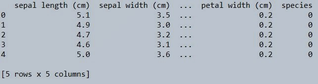
Figure 1 : Iris data Set top 5 record using the head function
Now lets perform some basic operations to know if the following dataset has null or Nan values.
iris_df.info()
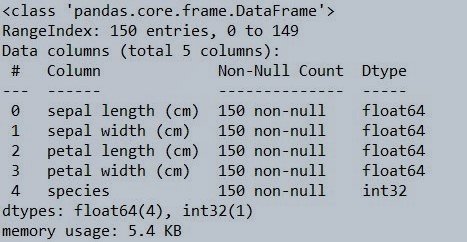
Figure 2 : Use the info function to check the iris data set for null values
iris_df.shape
(150, 5)
iris_df.isnull().any()
sepal length (cm) False
sepal width (cm) False
petal length (cm) False
petal width (cm) False
species False
dtype: bool
Now we will split the dataset into train and test. Train will have 80% of the data and test will have 20% of the data from the iris dataset. Simultaneously we will be creating another set with 50% of train data and 50% as test.
# Seggregate the features and target into seperate objects
X = iris_df.iloc[:,0:4]
Y = iris_df.iloc[:,4]
# Splitting the data - 80:20 ratio
X_train_1, X_test_1, Y_train_1, Y_test_1 = train_test_split(X , Y, test_size = 0.2, random_state = 42)
print("Training set 1 split input- ", X_train_1.shape)
print("Testing set 1 split input- ", X_test_1.shape)
# Splitting the data - 50:50 ratio
X_train_2, X_test_2, Y_train_2, Y_test_2 = train_test_split(X , Y, test_size = 0.5, random_state = 42)
print("Training set 2 split input- ", X_train_2.shape)
print("Testing set 2 split input- ", X_test_2.shape)
Training set 1 split input- (120, 4)
Testing set 1 split input- (30, 4)
Training set 2 split input- (75, 4)
Testing split 2 input- (75, 4)
We will now build the decision tree model on the train data set. Later we would be testing the model on the test data set. As of now, we have kept the train data set at 80% which is ideally not a good proportion. Decision trees have a drawback of over fitting on the data. Ideally in situations like this we should feed a relatively lower proportion of data as training data. But, the objective over here is to simulate and check the results.
# Defining the decision tree algorithm
decisiontree_1 = DecisionTreeClassifier(random_state=0)
# Training the DT Algorithm on first train set
decisiontree_1.fit(X_train_1, Y_train_1)
# Defining the decision tree algorithm
decisiontree_2 = DecisionTreeClassifier(random_state=0)
# Training the DT Algorithm on second train set
decisiontree_2.fit(X_train_2, Y_train_2)
Now we will predict the accuracy of model on the respective test datasets.
# Predicting the values for the first data set
y_pred_decisiontree_1 = decisiontree_1.predict(X_test_1)
print("Classification report for first model- \n", classification_report(Y_test_1,y_pred_decisiontree_1))
# Predicting the values for the second data set
y_pred_decisiontree_2 = decisiontree_2.predict(X_test_2)
print("Classification report for second model- \n", classification_report(Y_test_2,y_pred_decisiontree_2))
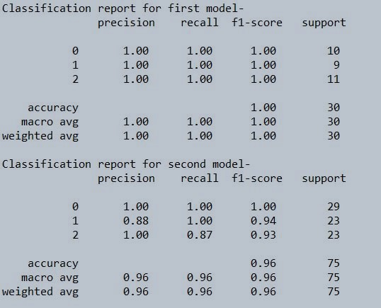
Figure 3 : Classification report for decision tree model
As we can see , the efficiency of a decision tree is higher than 90% even if we give it 50% training data. In real production environment, because of complexities and variation in the feature values, this may differ. Also one important aspect of a decision tree is its tendency to overlearn from the data. As a precaution, its always good to feed it with substantially reduced instances of learning data sets. You can use grid search to optimize your ML models, have a look at this implementation for reference on how to use grid search in Machine Learning using python GridSearchCV.
About the Author's:
Write A Public Review