
How to do Ridge Regression in Python ?
Table of Content
Introduction
Origin of Multicollinearity
Regression Model
Standardization
Ridge Regression Assumptions
Implementing Ridge Regression using python
Conclusion and Summary
Introduction
Ridge regression is a model which is used to analyze data which suffers multicollinearity. When this multicollinearity occurs, least squares are unbiased and the variances are large making the predicted values to be far from the actual values. The ridge regression standard error can be reduced by adding a degree to the bias. The effect of multicollinearity can result to wrong estimate of regression coefficient and also can increase the standard errors of regression coefficient. It performs L2 regularization.
Origin of Multicollinearity
Data Collection- It can cause multicollinearity
Outliers- Extreme values can cause multicollinearity
Over defined model – Variable count are more than the observation count
Regression Model
The basic equation for any type of regression is
Y=XB + e
In which,
Y represent dependent variable,
X represents independent variable,
B represent regression coefficient which will be calculated later and
lastly e represents errors which are residuals.
Standardization
While performing ridge regression the first step is to standardize the variables in dataset on which you are working. Standardization is done by subtracting their means and dividing it with standard deviation. This is performed on both dependent and independent variables which are there in the dataset. All the calculations done are based on standardise value. When we set the final regression coefficient, the standardized variables are converted back to the original scale.
Ridge Regression Assumptions
The assumption in ridge regression is same as assumption in linear regression which is constant variance, independence and linearity. Normality should not be assumed as ridge regression does not provide confidence limit.
Implementing Ridge Regression using Python
For better understanding of ridge regression, we will look at the following example performed in python.
First Import all the required libraries
    from sklearn.datasets import make_regression
    from matplotlib import pyplot as pltplt
    import numpy as npnp
    from sklearn.linear_model import Ridge
For explaining purpose, we will create a sample dataset using scikit -learn which will match the regression.
    L, g, coefficient = make_regression(
    n_samples=50,
    n_features=1,
    n_informative=1,
    n_targets=1,
    noise=5,
    coef=True,
    random_state=1
)
Regularization
Here we will define the hyperparameter which is alpha. alpha defines the strength of the regularization. the larger the value of alpha the greater the strength of the regularization. it means that the bias of the model will be high when the alpha value will be high. when we set the alpha value to 1 i.e., alpha =1 then the model will act similar to linear regression model.
    alpha_alpha = 1
    n, m = L.shape
    Id = npnp.identity(m)
    z = npnp.dot(npnp.dot(npnp.linalg.inv(npnp.dot(L.T, L) + alpha_alpha * Id), L.T), g)
and also we solve for z using the equation mentioned above.
when we compare z and actual coefficient which is used in generating data, we can see that they are not equal to each other but are very close to each other
    z
array([87.37153533])

    coefficient
array(90.34019153)
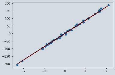
Now let see how the regression line will fit the data.
    pltplt.scatter(L, g)
    pltplt.plot(L, z*L, c='maroon')
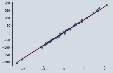
Now we will create and train instance of ridge class.
    rrrr = Ridge(alpha=1)
    rrrr.fit(L, g)
    z = rrrr.coef_
    z
array([87.39928165])
we get the same value of z where we solved it for linear algebra. So, the regression line will be similar to the one above.
    pltplt.scatter(L, g)
    pltplt.plot(L, z*L, c='maroon')
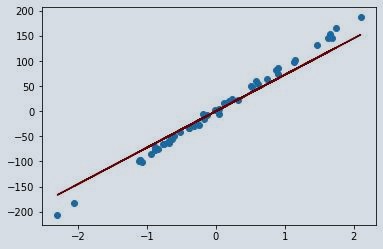
To see the effect of regularization hyperparameter i.e., alpha we can set the alpha value to whichever value we want to avoid overfitting or under fitting. Here I am taking alpha value as 11 and we will visualise it and will compare it to the previous one as well.
    rrrr = Ridge(alpha=11)
    rrrr.fit(L, g)
    z = rrrr.coef_[0]
    pltplt.scatter(L, g)
    pltplt.plot(L, z*L, c='maroon')
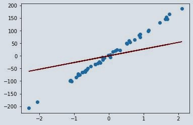
As we can see the regression line is no longer a perfect line for the dataset. we can say that ridge regression model has a higher bias compared to the one where we have taken alpha value as 1. For better understanding let’s take alpha value as 111 and lets visualise it. So, we can observe and compare the results.
    rrrr = Ridge(alpha=111)
    rrrr.fit(L, g)
    z = rrrr.coef_[0]
    pltplt.scatter(L, g)
    pltplt.plot(L, z*L, c='maroon')
Conclusion and Summary
When the alpha value moves towards positive infinity, the regression line will move towards a mean of 0. This happens because it minimizes the variance across different dataset. In this article, we studied ridge regression and had a look on the origin of multicollinearity. We also studied regression model and assumption of ridge regression as well. At last, we implemented ridge regression on the dataset and found out that it has better performance as compare to the simple regression model. You can learn more about linear regression by reading this article on How to implement Linear Regression in Python from Scratch.
About the Author's:
Lohansh Srivastava
Lohansh is a Data Science Intern at Simple & Real Analytics. As a data science enthusiast he loves contributing to open source in Machine Learning domain. He holds a Bachelors Degree in Computer Science.
Mohan Rai
Mohan Rai is an Alumni of IIM Bangalore , he has completed his MBA from University of Pune and Bachelor of Science (Statistics) from University of Pune. He is a Certified Data Scientist by EMC. Mohan is a learner and has been enriching his experience throughout his career by exposing himself to several opportunities in the capacity of an Advisor, Consultant and a Business Owner. He has more than 18 years’ experience in the field of Analytics and has worked as an Analytics SME on domains ranging from IT, Banking, Construction, Real Estate, Automobile, Component Manufacturing and Retail. His functional scope covers areas including Training, Research, Sales, Market Research, Sales Planning, and Market Strategy.
Table of Content
- Introduction
- Origin of Multicollinearity
- Regression Model
- Standardization
- Ridge Regression Assumptions
- Implementing Ridge Regression using python
- Conclusion and Summary
Ridge regression is a model which is used to analyze data which suffers multicollinearity. When this multicollinearity occurs, least squares are unbiased and the variances are large making the predicted values to be far from the actual values. The ridge regression standard error can be reduced by adding a degree to the bias. The effect of multicollinearity can result to wrong estimate of regression coefficient and also can increase the standard errors of regression coefficient. It performs L2 regularization.
- Data Collection- It can cause multicollinearity
- Outliers- Extreme values can cause multicollinearity
- Over defined model – Variable count are more than the observation count
The basic equation for any type of regression is
Y=XB + e
In which,
Y represent dependent variable,
X represents independent variable,
B represent regression coefficient which will be calculated later and
lastly e represents errors which are residuals.
While performing ridge regression the first step is to standardize the variables in dataset on which you are working. Standardization is done by subtracting their means and dividing it with standard deviation. This is performed on both dependent and independent variables which are there in the dataset. All the calculations done are based on standardise value. When we set the final regression coefficient, the standardized variables are converted back to the original scale.
The assumption in ridge regression is same as assumption in linear regression which is constant variance, independence and linearity. Normality should not be assumed as ridge regression does not provide confidence limit.
For better understanding of ridge regression, we will look at the following example performed in python.
- First Import all the required libraries
from sklearn.datasets import make_regression
from matplotlib import pyplot as pltplt
import numpy as npnp
from sklearn.linear_model import Ridge
- For explaining purpose, we will create a sample dataset using scikit -learn which will match the regression.
L, g, coefficient = make_regression(
n_samples=50,
n_features=1,
n_informative=1,
n_targets=1,
noise=5,
coef=True,
random_state=1
)
- Regularization
Here we will define the hyperparameter which is alpha. alpha defines the strength of the regularization. the larger the value of alpha the greater the strength of the regularization. it means that the bias of the model will be high when the alpha value will be high. when we set the alpha value to 1 i.e., alpha =1 then the model will act similar to linear regression model.
alpha_alpha = 1
n, m = L.shape
Id = npnp.identity(m)
z = npnp.dot(npnp.dot(npnp.linalg.inv(npnp.dot(L.T, L) + alpha_alpha * Id), L.T), g)
and also we solve for z using the equation mentioned above.
when we compare z and actual coefficient which is used in generating data, we can see that they are not equal to each other but are very close to each other
z
array([87.37153533])
coefficient
array(90.34019153)
- Now let see how the regression line will fit the data.
pltplt.scatter(L, g)
pltplt.plot(L, z*L, c='maroon')
- Now we will create and train instance of ridge class.
rrrr = Ridge(alpha=1)
rrrr.fit(L, g)
z = rrrr.coef_
z
array([87.39928165])
we get the same value of z where we solved it for linear algebra. So, the regression line will be similar to the one above.
pltplt.scatter(L, g)
pltplt.plot(L, z*L, c='maroon')
To see the effect of regularization hyperparameter i.e., alpha we can set the alpha value to whichever value we want to avoid overfitting or under fitting. Here I am taking alpha value as 11 and we will visualise it and will compare it to the previous one as well.
rrrr = Ridge(alpha=11)
rrrr.fit(L, g)
z = rrrr.coef_[0]
pltplt.scatter(L, g)
pltplt.plot(L, z*L, c='maroon')
As we can see the regression line is no longer a perfect line for the dataset. we can say that ridge regression model has a higher bias compared to the one where we have taken alpha value as 1. For better understanding let’s take alpha value as 111 and lets visualise it. So, we can observe and compare the results.
rrrr = Ridge(alpha=111)
rrrr.fit(L, g)
z = rrrr.coef_[0]
pltplt.scatter(L, g)
pltplt.plot(L, z*L, c='maroon')
When the alpha value moves towards positive infinity, the regression line will move towards a mean of 0. This happens because it minimizes the variance across different dataset. In this article, we studied ridge regression and had a look on the origin of multicollinearity. We also studied regression model and assumption of ridge regression as well. At last, we implemented ridge regression on the dataset and found out that it has better performance as compare to the simple regression model. You can learn more about linear regression by reading this article on How to implement Linear Regression in Python from Scratch.
About the Author's:
Write A Public Review