
Table of Content:
Introduction
- Ever wondered what parameters value to choose as an input for model?
- What should be the maximum depth for decision tree?
- How many trees should be in random forest?
- How many layers should I have in neural network layer or number of neurons in layers?
- What should be the learning rate for model?
And many more questions like this could be answered by Hyperparameter Tuning.
So now the question arises what is Hyperparameter. Basically, it’s a set of parameters which are set to optimize or to get the best performance by model. Now, we don’t know at which values of parameters model will give best result, so we tune the parameters to get optimum result. So we can say that process of finding the combination of hyperparameters which reduces the predefined loss functions and increases the accuracy of given data is known as Hyperparameter Tuning.
Types of Hyperparameter Tuning
We can tune the model by following methods:
- Manual Search
- Grid Search CV
- Randomized Search CV
Manual Search Hyperparameter Tuning
As the name indicates, the process of tuning the hyperparameters manually by trial and error method and by experience is known as Manual Search tuning.
This process is repeated until we don’t get the best hyperparameters which increases the accuracy of model.
Grid Search CV
In Grid Search CV, model is build on every combination of given various hyperparameters and evaluate each model and gives the hyperparameters which have the highest accuracy.
In this technique each set of parameters are considered and model accuracy is noted. The set of parameters which give the highest accuracy is considered to build the model.
Read more about Grid Search in Python here.
Randomized Search CV
In Randomized Search CV, hyperparameters combination are taken randomly to find the best solution for building the model.
As it takes random values, it is faster than grid search cv but gives less accuracy than grid search cv.
Implementation of Randomized Search CV
    # Importing Libraries
    import numpy as np
    import pandas as pd
    import matplotlib.pyplot as plt
    import seaborn as sns
    import warnings
    from sklearn.model_selection import train_test_split
    from sklearn.linear_model import LogisticRegression
    from sklearn.ensemble import RandomForestRegressor
    from sklearn.tree import DecisionTreeRegressor
    from xgboost import XGBRegressor
    from sklearn.model_selection import RandomizedSearchCV
    from scipy.stats import randint
    from xgboost import XGBRegressor
    from sklearn.metrics import accuracy_score , r2_score
    from imblearn.over_sampling import SMOTE
    from sklearn.preprocessing import StandardScaler
    warnings.filterwarnings('ignore')
    # Importing Dataset
    # Download red wine quality and white wine quality, sourced from UCI Machine Learning Archive
    red = pd.read_csv('winequality-red.csv', sep = ';')
    white = pd.read_csv('winequality-white.csv',sep=';')

    red.head(5)

   fixed acidity  volatile acidity  citric acid  ...  sulphates  alcohol  quality
0            7.4              0.70         0.00  ...       0.56      9.4        5
1            7.8              0.88         0.00  ...       0.68      9.8        5
2            7.8              0.76         0.04  ...       0.65      9.8        5
3           11.2              0.28         0.56  ...       0.58      9.8        6
4            7.4              0.70         0.00  ...       0.56      9.4        5

    white.head()

   fixed acidity  volatile acidity  citric acid  ...  sulphates  alcohol  quality
0            7.0              0.27         0.36  ...       0.45      8.8        6
1            6.3              0.30         0.34  ...       0.49      9.5        6
2            8.1              0.28         0.40  ...       0.44     10.1        6
3            7.2              0.23         0.32  ...       0.40      9.9        6
4            7.2              0.23         0.32  ...       0.40      9.9        6
    # Combining both data
    red['Type'] = 'Red'
    white['Type'] = 'White'

    df = pd.concat([red,white], axis=0)
    df.head(5)

   fixed acidity  volatile acidity  citric acid  ...  alcohol  quality  Type
0            7.4              0.70         0.00  ...      9.4        5     1
1            7.8              0.88         0.00  ...      9.8        5     1
2            7.8              0.76         0.04  ...      9.8        5     1
3           11.2              0.28         0.56  ...      9.8        6     1
4            7.4              0.70         0.00  ...      9.4        5     1
    df.describe()

       fixed acidity  volatile acidity  ...      quality         Type
count    6497.000000       6497.000000  ...  6497.000000  6497.000000
mean        7.215307          0.339666  ...     5.818378     0.246114
std         1.296434          0.164636  ...     0.873255     0.430779
min         3.800000          0.080000  ...     3.000000     0.000000
25%         6.400000          0.230000  ...     5.000000     0.000000
50%         7.000000          0.290000  ...     6.000000     0.000000
75%         7.700000          0.400000  ...     6.000000     0.000000
max        15.900000          1.580000  ...     9.000000     1.000000
    df.info()

Int64Index: 6497 entries, 0 to 4897
Data columns (total 13 columns):
 #   Column                Non-Null Count  Dtype
---  ------                --------------  -----
 0   fixed acidity         6497 non-null   float64
 1   volatile acidity      6497 non-null   float64
 2   citric acid           6497 non-null   float64
 3   residual sugar        6497 non-null   float64
 4   chlorides             6497 non-null   float64
 5   free sulfur dioxide   6497 non-null   float64
 6   total sulfur dioxide  6497 non-null   float64
 7   density               6497 non-null   float64
 8   pH                    6497 non-null   float64
 9   sulphates             6497 non-null   float64
 10  alcohol               6497 non-null   float64
 11  quality               6497 non-null   int64
 12  Type                  6497 non-null   int64
dtypes: float64(11), int64(2)
memory usage: 710.6 KB
    # check missing values
    df.isnull().sum()

fixed acidity           0
volatile acidity        0
citric acid             0
residual sugar          0
chlorides               0
free sulfur dioxide     0
total sulfur dioxide    0
density                 0
pH                      0
sulphates               0
alcohol                 0
quality                 0
Type                    0
dtype: int64
    df['Type'].value_counts()

white    4898
red      1599
Name: Type, dtype: int64
    df['quality'].value_counts()

6    2836
5    2138
7    1079
4     216
8     193
3      30
9       5
Name: quality, dtype: int64
As we can see, the data is imbalanced, we will have to handle this later.
    # correlation between features
    corr = df.corr(method='spearman')
    plt.figure(figsize=(20,10))
    sns.heatmap(corr, annot=True)
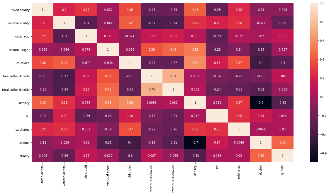
Figure 1 : Correlation plot for selecting best variables
From heatmap in Figure 1, it is clear that the most correlated features with quality are alcohol, density, free sulfur dioxide, chloride and citric acid.
    # Splitting the dataset
    X = df[['alcohol', 'density', 'free sulfur dioxide', 'chlorides','citric acid']]
    y = df['quality']

    # Balancing the dataset
    oversample = SMOTE(k_neighbors=4)
    # transform the dataset
    X, y = oversample.fit_resample(X, y)

    # Split into train and test sets
    X_train,X_test,y_train,y_test = train_test_split(X,y, test_size=0.25, random_state=42)

    # Feature Scaling
    scaler = StandardScaler()
    scaler.fit(X)
    X_train = scaler.transform(X_train)
    X_test = scaler.transform(X_test)
    # Build the Logistic model
    lr = LogisticRegression()
    lr.fit(X_train,y_train)
    lr_pred = lr.predict(X_test)
    r2_score(lr_pred,y_test)

0.46038027394992365
    # Build the Random Forest Model
    from sklearn.ensemble import RandomForestRegressor
    rf = RandomForestRegressor()
    rf.fit(X_train,y_train)
    rf_pred = rf.predict(X_test)
    r2_score(rf_pred,y_test)

0.916805568147207
    # Build Decision Tree Model
    dt = DecisionTreeRegressor()
    dt.fit(X_train,y_train)
    pred_dt = dt.predict(X_test)
    r2_score(pred_dt,y_test)

0.8533160326226503
    # Build XGBoost Model
    xgb = XGBRegressor()
    xgb.fit(X_train,y_train)
    xg_pred = xgb.predict(X_test)
    r2_score(xg_pred,y_test)

0.8705397134271582
Accuracy Score of Random Forest Regressor Model is 91.68%. Now, let’s tune the hyperparameters and see how its effect the accuracy of model.
    # Hyperparameter Tuning
    rs = {'n_estimators': [100,150,200,300],
          'max_features': ['auto', 'sqrt'],
          'max_depth': [10, 20, 40, 50, 60, 80, 100, None],
          'min_samples_leaf': randint(1,8),
          'bootstrap': [True,False]}

    random_rf = RandomizedSearchCV(estimator = rf, param_distributions = rs, n_iter = 100, cv = 3, verbose=2, random_state=42, n_jobs = -1)
    # Fit the random search model
    random_rf.fit(X_train, y_train)

RandomizedSearchCV(cv=3, estimator=RandomForestRegressor(), n_iter=100,
                   n_jobs=-1,
                   param_distributions={'bootstrap': [True, False],
                                        'max_depth': [10, 20, 40, 50, 60, 80,
                                                      100, None],
                                        'max_features': ['auto', 'sqrt'],
                                        'min_samples_leaf': ,
                                        'n_estimators': [100, 150, 200, 300]},
                   random_state=42, verbose=2)
    random_rf.best_params_

{'bootstrap': False,
 'max_depth': 50,
 'max_features': 'sqrt',
 'min_samples_leaf': 1,
 'n_estimators': 300}
    random_rf.best_estimator_

RandomForestRegressor(bootstrap=False, max_depth=50, max_features='sqrt', n_estimators=300)
    rf1 = RandomForestRegressor(bootstrap=False, ccp_alpha=0.0, criterion='mse',
                          max_depth=50, max_features='sqrt', max_leaf_nodes=None,
                          max_samples=None, min_impurity_decrease=0.0,
                          min_impurity_split=None, min_samples_leaf=1,
                          min_samples_split=2, min_weight_fraction_leaf=0.0,
                          n_estimators=300, n_jobs=None, oob_score=False,
                          random_state=None, verbose=0, warm_start=False)

    rf1.fit(X_train,y_train)

RandomForestRegressor(bootstrap=False, max_depth=50, max_features='sqrt',
                      n_estimators=300)
    rf_pr = rf1.predict(X_test)
    r2_score(rf_pr,y_test)

0.9322745287584387
Conclusion
With the help of hyperparameter tuning models accuracy increased by 2% and now it is 93.22%.
Randomized Search CV is faster than Grid Search CV. So, for big data we can use Randomized Search CV instead of Grid Search but if higher accuracy is needed than we should go with Grid search.
About the Author's:
Write A Public Review